We decide to read the book Molecular Evolution: A Statistical Approach by Ziheng Yang, to gether on a weekly basis. Contents in this summary involve AI-generated text.
1. Models of nucleotide substitution
- We define $p$ distance as thr proportion of sites that differ between two sequences.
- The true evolutionary distance $d$ is the expected number of substitutions per site between two sequences.
- CTMC (Continuous Time Markov Chain): four nucleotides are states of the chain, it will reach to steady state with a stationary distribution, via a substitution rate matrix.
Markov models of nucleotide substitution and distance estimation
The JC69 model
- Jukes-Cantor 1969 model.
- The substitution rate matrix $Q$ is
\(Q = \begin{pmatrix}
-3\lambda & \lambda & \lambda & \lambda \\
\lambda & -3\lambda & \lambda & \lambda \\
\lambda & \lambda & -3\lambda & \lambda \\
\lambda & \lambda & \lambda & -3\lambda
\end{pmatrix}\)
- The matrix of transition probability: $P(t) = e^{Qt}$. This is using Kolmogorov forward/backward? equation, where $\frac{dP(t)}{dt} = QP(t)$.
- We then use Taylor expansion to get $P(t) = I + Qt + \frac{Q^2t^2}{2!} + \cdots$.
- Chapman–Kolmogorov equation: $P_ij(t+s) = \sum_k P_ik(t)P_kj(s)$. This account for the multiple (hidden) states between $i$ and $j$.
- As $d=3\lambda t$, then $p(d) = 3p_1(t)=\frac{3}{4}-\frac{3}{4}e^{-4\lambda t}=\frac{3}{4}-\frac{3}{4}e^{-4d/3}$, then $\hat{d}=-\frac{3}{4}log(1-\frac{4}{3}\hat{p})$.
The K80 model
- Kimura 1980 model.
- Transitions: pyrimidine (T $\leftrightarrow$ C), purine (A $\leftrightarrow$ G).
- Transversion: (T, C $\leftrightarrow$ A, G).
- $d = (\alpha + 2\beta)t$.
- $\kappa = \frac{\alpha}{\beta}$.
- $E(S) = p_1(t)$.
- $E(V) = 2p_2(t)$.
- $\hat{d} = -\frac{1}{2} \log(1 - 2S - V) - \frac{1}{4} \log(1 - 2V)$.
HKY85, F84, TN93, etc.
TN93
- Tamura-Nei 1993 model.
- 7 parameters and 6 free parameters.
- $\pi_Y = \pi_T + \pi_C$ and $\pi_R = \pi_A + \pi_G$.
- $P(t)$ can be solved using spectral decomposition of $Q$.
- $Q = U \Lambda U^{-1}$.
- $\Lambda = \text{diag}\lbrace \lambda_1, \lambda_2, \lambda_3, \lambda_4 \rbrace$.
- $P(t) = U e^{\Lambda t} U^{-1} = U \text{diag}\lbrace e^{\lambda_1 t}, e^{\lambda_2 t}, e^{\lambda_3 t}, e^{\lambda_4 t} \rbrace U^{-1}$.
- Essense of linear algebra by 3Blue1Brown.
- $\lambda = -\sum_i \pi_i q_{ii} = 2\pi_T \pi_C \alpha_1 + 2\pi_A \pi_G \alpha_2 + 2\pi_Y \pi_R \beta$.
- $d = \lambda t$.
- Using $E(S_1), E(S_2), E(V)$ to estimate $\alpha_1, \alpha_2, \beta$.
- $\hat{d}$ can be represented as a function of nucleotide frequencies and $E(S_1), E(S_2), E(V)$.
HKY85 and F84
The transition/transversion rate ratio
- Three definitions:
- $E(S)/E(V) = p_1(t)/2p_2(t)$ under the K80 model (the uncorrected method).
- $\kappa = \alpha/\beta$ under the K80 model (corrected).
- $R = \alpha/2\beta$ under the K80 model (corredted). It’s called average transition/transversion ratio. More generally, $R = \frac{\pi_T q_{TC} + \pi_C q_{CT} + \pi_A q_{AG} + \pi_G q_{GA}}{\pi_T q_{TA} + \pi_T q_{TG} + \pi_C q_{CA} + \pi_C q_{CG} + \pi_A q_{AT} + \pi_A q_{AC} + \pi_G q_{GT} + \pi_G q_{GC}}$ under UNREST.
Variable substitution rates among sites
- Assuming the rate $r$ for any site is drawn from a gamma distribution.
- Models with Gamma distance denoted by a suffix ‘$+\Gamma$’.
- Gamma distribution have two parameters: shape $\alpha$ and scale $\beta$. The mean is $\alpha/\beta$, and the variance is $\alpha/\beta^2$. You can also consider them as number of Poisson process events of $\alpha$ with rate $1/\beta$.
- Note that the gamma distribution here sets $\alpha = \beta$ so that the mean equals to $1$.
- If a site has a rate $r$, the distance between sequences becomes $d = r t$.
- $p(d\cdot r)$ can be calculated by integrating the gamma distribution.
- For JC69 model, $p = \int_0^\infty \left( \frac{3}{4} - \frac{3}{4} e^{-4d \cdot r / 3} \right) g(r) \, dr
= \frac{3}{4} - \frac{3}{4} \left( 1 + \frac{4d}{3\beta} \right)^{-\alpha}$.
- Similarly, one can derive a gamma distance under virtually every model for which a one-rate distance formula is available.
- It is well known that ignoring rate variation among sites leads to underestimation of both the sequence distance and the transition/transversion rate ratio.
Maximum likelihood estimation of distance
- The likelihood function is $L(\theta; X) = f(X\vert\theta)$.
- MLE is the value of $\theta$ that maximizes the likelihood function.
- Probability vs. Likelihood:
- Likelihood $\ne$ Probability: Likelihood does not sum to 1, unlike probability.
- Interpretation: Probability is understood by area under the curve, while likelihood is compared at specific points.
- Reparametrization: Likelihood is invariant under monotonic transformations, so MLEs remain unchanged.
- Nonlinear Effects: Nonlinear transformations alter probability density shapes, potentially changing modality.
The JC69 model
- The single parameter is the distance $d = 3\lambda t$. The data are two aligned sequences, each $n$ sites long, with $x$ differences.
- $p = 3p_1(t) = \frac{3}{4} - \frac{3}{4} e^{-4d/3}$.
- The likelihood function is $L(d; X) = {n\choose x}p^x(1-p)^{n-x}$.
- After reparametrization: $L(d; X) = (\frac{1}{4}p_1)^x (\frac{1}{4}p_0)^{n-x}$. (I think $\frac{1}{4}$ can be further dropped.)
- Two approaches to estimate confidence intervals:
- Normal approximation: $\hat{d} \pm 1.96 \sqrt{var({d})}$.
- Likelihood interval, based on likelihood ratio test: $\frac{1}{2}\chi^2_{1, 5\%} = 3.841/2 = 1.921$.
The K80 model
- $L(d, \kappa; n_S, n_V) = \left( \frac{p_0}{4} \right)^{(n - n_S - n_V)} \times \left( \frac{p_1}{4} \right)^{n_S} \times \left( \frac{p_2}{4} \right)^{n_V}.$
- $\frac{1}{2}\chi^2_{2, 5\%} = 5.991/2 = 2.995$.
Likelihood ratio test of substitution models
- For model comparison, if two models are nested, then the likelihood ratio test can be used.
Profile and integrated likelihood
- The above approaches, estimating one parameter while ignoring the other, are called relative likelihood, pseudo likelihood or estimated likelihood.
- A more respective approach is profile likelihood.
- $\ell(d) = \ell(d, \hat{\kappa}_d)$, where $\hat{\kappa}_d$ is the MLE of $\kappa$ for the given $d$.
- This is a pragmatic approach that most often leads to reasonable answers.
- Integrated likelihood or marginal likelihood is the likelihood of the data given the model, averaged over the parameter space.
- It is possible to use a improper prior, such as a uniform distribution, to calculate the marginal likelihood.
- Integrated likelihood is always smaller than the profile likelihood.
Markov chains and distance estimation under general models
Distance under the unrestricted (UNREST) model
- Unlike the GTR model, UNREST does not assume time-reversibility.
- Here we consider a strand-symmetry model, where $q_{TC} = q_{AG}$.
- Equilibrium nucleotide frequencies ${\pi_T, \pi_C, \pi_A, \pi_G}$ perhaps by coincidence, can be estimated analytically.
- Identifiability Issues and Distance Calculation
- The model can, in theory, identify the root of a two-sequence tree.
- However, estimating both $t_1$ and $t_2$ separately leads to high correlation between estimates.
- The model has 13 parameters:
- 11 rate parameters in $Q$.
- 2 branch lengths $t_1, t_2$.
- Challenges:
- No analytical solution for MLEs.
- Complex eigenvalues make numerical estimation difficult.
- Many datasets do not provide enough information to estimate so many parameters.
- *Conclusion:-
- Although $t_1$ and $t_2$ are identifiable, their estimates are highly correlated.
- The UNREST model is not recommended for distance calculations.
Distance under the general time-reversible model
- Time-Reversibility in Markov Chains
- A Markov chain is time-reversible if:
\(\pi_i q_{ij} = \pi_j q_{ji}, \quad \text{for all } i \neq j.\)
This condition is known as detailed balance.
- Reversibility is a mathematical convenience, not necessarily a biological property.
- Models such as JC69, K80, F84, HKY85, and TN93 are all time-reversible.
- Rate Matrix for GTR Model
- The GTR (General Time-Reversible) model is defined using the rate matrix:
\(Q =
\begin{bmatrix}
\cdot & a\pi_C & b\pi_A & c\pi_G \\
a\pi_T & \cdot & d\pi_A & e\pi_G \\
b\pi_T & d\pi_C & \cdot & f\pi_G \\
c\pi_T & e\pi_C & f\pi_A & \cdot
\end{bmatrix}\)
- It has nine free parameters (six substitution rates + three equilibrium frequencies).
- Simplification of Likelihood Computation
- Reversibility simplifies likelihood computation:
\(f_{ij}(t_1, t_2) = \sum_k \pi_k p_{ki}(t_1) p_{kj}(t_2) = \pi_i p_{ij}(t_1 + t_2).\)
- The second equality follows from reversibility.
- The third equality follows from the Chapman-Kolmogorov theorem.
- This allows estimation of total branch length instead of individual times.
- Log-Likelihood Formulation
- The log-likelihood function is:
\(\ell(t, a, b, c, d, e, f, \pi_T, \pi_C, \pi_A) = \sum_i \sum_j n_{ij} \log(\pi_i p_{ij}(t)).\)
- After scaling, the distance is defined as:
\(d = -t \sum_i \pi_i q_{ii} = t.\)
- Note that distance formulae are not MLEs.
- Observed base frequencies are not MLEs of the base frequency parameters.
- All 16 site patterns have distinct probabilities in the likelihood function but are collapsed in distance formulae (e.g., TT, CC, AA, GG).
- Despite this simplification, distance formulae still approximate MLEs well.
- Pairwise comparisons sum up branch lengths but may overestimate distances.
- Likelihood-based methods (ML, Bayesian) provide better phylogenetic estimates.
2. Models of amino acid substitution and codon substitution
Models of amino acid replacement
Empirical models
- Empirical models:
- The rates of substitution are estimated directly from observed sequence variations, without explicitly considering the biological processes that drive these substitutions.
- They are statistical and data-driven, without needing detailed knowledge of the underlying biological mechanisms.
- Mechanistic models:
- They are based on the underlying biological processes that drive sequence evolution.
- They offer more interpretative power, helping to understand the biological mechanisms and evolutionary forces that shape protein sequences.
- Empirical models of amino acid substitution are all constructed by estimating the relative substitution rates between amino acids under the GTR model.
- Under GTR, $\pi_i q_{ij} = \pi_j q_{ji}$ and $\pi_i p_{ij}(t) = \pi_j p_{ji}(t)$, with $i,j \in {1,2,\ldots,20}$.
- $q_{ij}$ or $s_{ij}$ are the amino acid exchangeabilities.
- Dayhoff (1978) and JTT (1992): fixed estimates.
- Dayhoff+F, JTT+F, add 19 free parameters by replacing the $\pi_i$
in the empirical matrices by the frequencies estimated from the data.
- WAG (2001), LG (2008) etc. use maximum likelihood to estimate the exchangeabilities.
- BLOSUM (1992) focus on more conserved regions in protein families.
- BLOSUM62 is often considered roughly equivalent to PAM250.
- Some features in the estimated exchangeabilities are in fact as expected from the physico-chemical properties of amino acids. Also the larger number of substitution events needed to change between two amino acids, the lower the exchangeability. Evidence by comparing the exchangeabilities in normal proteins and mitochondrial proteins (codon table is different).
Mechanistic models
- Yang et al. (1998) implemented a few mechanistic models, taking account of e.g. different mutation rates between nucleotides, translation of the codon triplet into amino acid, and acceptance or rejection of the amino acid due to selective pressure on the protein.
- The improvement was not extraordinary, perhaps reflecting our poor understanding of which of the many chemical properties are most important and how they affect amino acid substitution rates
Among-site heterogeneity
- Dayhoff+$\Gamma$, JTT+$\Gamma$, etc. are similar to the nucleotide models with among-site rate variation. $rQ$ is the rate matrix for a site.
- Recall that in the Gamma model, we delibrately set $\alpha = \beta$ so that the mean is 1. The higher the $\alpha$, the more concentrated the distribution is around the mean.
- Site-specific amino acid frequency parameters is also possible. For each (group of) site, this reflects how likely different amino acids are to appear (different patterns). However, this approach adds many parameters, making it challenging for maximum likelihood (ML) analysis.
Estimation of distance between two protein sequences
The Poisson model
- The number of substitutions over time $t$ can be a Poisson-disributed random variable under rate $\lambda$.
- Similar to JC69 model, the expected number of substitutions is $d = 19\lambda t$.
- Similarly, the expected distance is $\hat{d} = -\frac{19}{20}\log(1-\frac{20}{19}\hat{p})$. If $p > \frac{19}{20}$, then $\hat{d} = \infty$.
Empirical models
- We deliberately set $-\sum_i \pi_i q_{ii} = 1$ so that $d = 1 \times t$, the mean distance is 1.
- Under GTR, the log-likelihood function is $\ell(t) = \sum_i \sum_j n_{ij} \log(\pi_i p_{ij}(t))$.
- We can also use $p$ distance, $p = 1 - \sum_i \pi_i p_{ii}(t)$, but this will lose information, nevertheless, should approximate the MLE well.
Gamma distance
- Under something similar to JC69, adding a gamma distribution to the rate of substitution, we have $\hat{d} = \frac{19}{20} \alpha [(1 - \frac{20}{19}\hat{p})^{-\frac{1}{\alpha}} - 1]$. This is obtained by integration of the gamma distribution over the formula for $p$ distance (see formula 1.35).
- For empirical models, use ML to estimate the distance.
Models of codon substitution
The basic model
- The instantaneous rate matrix $Q$ is a $61 \times 61$ matrix.
-
\[q_{IJ} = \begin{cases}
0, & \text{if I and J differ at two or three codon positions,} \\
\pi_J, & \text{if I and J differ by a synonymous transversion,} \\
\kappa\pi_J, & \text{if I and J differ by a synonymous transition,} \\
\omega\pi_J, & \text{if I and J differ by a nonsynonymous transversion,} \\
\omega\kappa\pi_J, & \text{if I and J differ by a nonsynonymous transition.}
\end{cases}\]
- $\omega$ is the nonsynonymous/synonymous rate ratio. If $\omega > 1$, it indicates positive selection, if $\omega < 1$, it indicates purifying selection.
- Fequal model: $\pi_i = 1/61$.
- F1x4 model, F3x4 model, and F61 model: $\pi_i$ are estimated from the data.
- The rate matrix $Q$ time-reversible as it meets the detailed balance condition.
Variations and extensions
- The Muse-Gaut model (1994) is a generalization of the basic model.
- Simialr to F3x4 with omega?
- The mutation-selection (FMutSel) model.
- mutation bias: $\mu_{ij} = a_{ij} \pi^*_j$.
- selection: $S_{IJ} = f_J - f_I$.
- The probability of fixation of the mutation is $P_{IJ} = \frac{2S_{IJ}}{1 - e^{-2NS_{IJ}}}$.
- The $\omega$ ratio does not have to be a single parameter, it can be modelled by physico-chemical properties, e.g. $\omega_{IJ} = ae^{-bd_{IJ}}$, where $d_{IJ}$ is the chemical distance between amino acids.
- Or you can model $\omega$ by a few pre-specified categories of nonsynonymous substitutions.
- Allowing double or triple mutations should be more realistic. It is common to observe ‘synonymous’ differences between the two sets of serine codons (TCN and AGY) which cannot exchange by a single nucleotide mutation. Some people argue this is because separate lines of descent rather than multiple mutations.
Estimation of $d_S$ and $d_N$
- Recall that the evolutionary distance $d$ focuses on the entire sequence, now we want to separate the distance by synonymous and nonsynonymous mutations, then we get $d_S$ and $d_N$.
- Definitions: The number of synonymous/nonsynonymous substitutions per synonymous/nonsynonymous site.
- Methods: Counting and ML.
Counting methods
- Three steps:
- Count the number of synonymous and nonsynonymous sites.
- Count the number of synonymous and nonsynonymous differences.
- Calculate the proportions of differences and correct for multiple hits.
- A basic model is Nei and Gojobori (1986) (NG86), which used equal weights for all codon positions.
Counting sites ($S$ and $N$)
- Introducing NG86 model, then relax the model with unequal transition and transversion rates and
unequal codon usage. Different methods often produce very different estimates.
- There are three sites in a codon, and nine immediate neighbors.
- To calculate the synonymous and nonsynonymous sites, we need to multiply the synonymous/nonsynonymous probabilities (from the nine neighbors) by 3 sites. (Check Table 2.5)
Counting differences ($S_d$ and $N_d$)
- If two codons only differ by one nucleotide, then it is trivial to count the synonymous and nonsynonymous differences. (Check Table 2.6)
- If two codons differ by two or three nucleotides, there exist two or six possible paths to reach the codon, respectively.
- Weighting the paths needs knowledge.
Correcting for multiple hits
- We now have the $p$ distance, $p_S = S_d/S$ and $p_N = N_d/N$.
- The Jukes-Cantor correction is $d_S = -\frac{3}{4}\log(1 - \frac{4}{3}p_S)$ and $d_N = -\frac{3}{4}\log(1 - \frac{4}{3}p_N)$.
- This is logically flawed (Lewontin 1989), as JC69 assumes equal rates of substitution for all three other nucleotides, but when focusing on synonymous/nonsynonymous sites only, each nucleotide does not have three other nucleotides to change into.
Transition–transversion rate difference and codon usage
- From codon table, we see transitions at the third codon positions are more likely to be synonymous than transversions are. Therefore, a higher transition/transversion rate can lead to more synonymous substitutions, not necessarily due to selection. Ignoring this can lead to underestimation of $S$ (not $S_d$) and overestimation of $N$, and overestimation of $d_S$ and underestimation of $d_N$.
- The below methods classified codon positions into nondegenerate, two-fold degenerate, and four-fold degenerate sites, based on the number of synonymous substitutions possible. Note that some of the codons in fact do not fall into these categories, different methods may have different ways to deal with them.
- LWL85 Method (Li, Wu, and Luo, 1985):
- Counts two-fold degenerate sites as 1/3 synonymous and 2/3 nonsynonymous under the assumption of equal mutation rates.
- The distances are calculated using the total numbers of sites in different degeneracy classes and the estimated transition and transversion counts.
- LPB93 Method (Li, Pamilo, and Bianchi, 1993):
- Adjusts for transition–transversion rate bias (which was ignored by 1/3 and 2/3 approximation in LWL85).
- Uses the transition distance at four-fold sites to estimate $d_S$ and an averaged transversion distance at nondegenerate sites for $d_N$.
- Assuming that the transition rate is the same at the two-fold and four-fold sites; the transversion rate is the same at the nondegenerate and two-fold sites.
- LWL85m Method:
- A refinement of LWL85 that replaces the 1/3 assumption with an estimated proportion ($\rho$) of two-fold degenerate sites that are synonymous.
- Uses the ratio of transition and transversion distances at four-fold sites to estimate $\kappa$ (transition/transversion rate ratio).
- Alternative Approaches:
- Ina (1995) proposed not partitioning sites by codon degeneracy but instead weighting transitions and transversions based on neighboring codons (See Table 2.5).
- Consideration of unequal codon frequencies was introduced by Yang and Nielsen (2000), as previous models assumed equal codon frequencies, which is unrealistic.
- Example 2.2 is useful for understanding the above calculations.
- In Table 2.8, we see S are larger in LWL85m and Ina95, as they accounted for underestimation of S by considering ts/tv ratio, but ironically, they led to even more biased results, because they did not consider codon usage bias at the same time.
Maximum likelihood methods
- Under the basic model for codon substitution, which is a GTR again.
- Parameters estimated:
- $t$ (sequence divergence time or distance),
- $\kappa$ (transition/transversion rate ratio),
- $\omega$ (nonsynonymous/synonymous rate ratio),
- Codon frequencies (either fixed or estimated from the data), can be Fequal, F1x4, F3x4, or F61.
- $d_S$ and $d_N$ are then computed based on these ML estimates.
- Refer to Table 2.8, the Fequal with $\kappa=1$ is similar to NG86, and Fequal with $\kappa$ estimated is similar to LWL85, LPB93 and Ina95.
- Note that incorporating the transition–transversion rate difference has had much greater effect on the numbers of sites ($S$ and $N$) than on the numbers of substitutions ($S_d$ and $N_d$).
Comparing methods
- Estimation Bias and Model Effects:
- Ignoring Transition–Transversion Rate Differences:
- Leads to underestimation of synonymous sites ($S$) and overestimation of nonsynonymous sites ($N$).
- Results in overestimation of $d_S$ and underestimation of $\omega = d_N/d_S$.
- Ignoring Unequal Codon Usage:
- Has the opposite effect compared to ignoring transition–transversion rates.
- Leads to overestimation of $S$ and underestimation of $d_S$, which in turn overestimates $ω$.
- Codon frequency biases can sometimes override the effects of transition–transversion biases.
- The NG86 method, which ignores both transition–transversion differences and codon usage, sometimes produces more reliable estimates than models that only accommodate transition–transversion biases but ignore codon usage.
- Effect of Model Assumptions on Similar Sequences:
- When sequences are highly similar, different methods can produce very different estimates.
- Unlike nucleotide models, where distance estimates converge at low sequence divergences, codon-based models remain highly sensitive to assumptions.
- Importance of Model Assumptions:
- At low or moderate sequence divergences, different (counting or ML) methods produce similar results if they share the same assumptions.
- However, different counting/likelihood methods produce highly variable results because of differnt assumptions (e.g., $\kappa = 1?$ and codon bias).
- Advantages of the Likelihood Method Over Counting Methods:
- Conceptual simplicity
- Counting methods struggle with different transition/transversion rates and unequal codon frequencies.
- Some counting methods attempt to estimate $\kappa$, but this is challenging.
- Counting methods rely on nucleotide-based corrections for multiple hits, which can be logically flawed (mentioned under formula 2.15).
- Likelihood methods incorporate these complexities naturally without requiring correction formulas.
- No need for manual classification of synonymous vs. nonsynonymous substitutions, as these are inferred probabilistically.
- Easier to Incorporate Realistic Codon Models
- Likelihood methods can incorporate sophisticated codon substitution models.
- Example: GTR-style mutation models or HKY85-type models can be used in likelihood calculations.
More distances and interpretation of the $d_N/d_S$ ratio
More distances based on the codon model
- Additional Distance Measures in the Codon Model
- Since we can get the expected number of substitutions from codon $i$ to codon $j$ over time $t$ is given by $\pi_i q_{ij} t$.
- We can calculate many other distances, not limited to $d_N$ and $d_S$, based on:
- Transition vs. transversion substitutions.
- Codon position-specific changes (first, second, third codon positions).
- Conservative or radical amino acid changes, etc.
- Distances at Different Codon Positions
- Distances at the first, second, and third codon positions can be calculated separately:
- $d_{1A}, d_{2A}, d_{3A}$ → After selection on the protein.
- $d_{1B}, d_{2B}, d_{3B}$ → Before selection on the protein (fixing $\omega = 1$).
- Distance $d_4$ (Four-Fold Degenerate Sites)
- $d_4$ represents substitutions at four-fold degenerate sites in the third codon position.
- Used as an approximation of the neutral mutation rate.
Estimation of $d_S$ and $d_N$ in comparative genomics
- Time Scale Matters
- Estimating $d_S$ and $d_N$ requires a balance—sequences should be neither too similar nor too divergent.
- If species are too distantly related, synonymous substitutions may reach saturation, making $d_S$ unreliable.
- Estimates of $d_S > 3$ should be treated with caution, as high divergence leads to indistinguishable evolutionary distances.
- Solutions for High Divergence
- A phylogenetic approach can break long evolutionary distances into shorter branches by including multiple species.
- Issues with Low Divergence
- When sequences are too similar (e.g., within the same species or bacterial strains), $d_N/d_S$ estimates become unreliable.
- Observed bias: $d_N/d_S$ tends to decrease with increasing divergence, possibly due to MLE biases and correlations between parameter estimates.
- In within-population comparisons, deleterious nonsynonymous mutations may persist longer before being removed by selection, inflating $d_N/d_S$ at short timescales.
3. Phylogenetic reconstruction: overview
3.1 Tree concepts
Terminology
- Nodes (vertices) and branches (edges).
- Molecular clock: the rate of evolution is constant over time; Midpoint rooting: the root is placed at the midpoint of the longest path between two tips.
- Newick format:
(A:0.1,B:0.2,(C:0.3,D:0.4):0.5); Nexus format: #NEXUS; BEGIN TREES; TREE tree1 = (A:0.1,B:0.2,(C:0.3,D:0.4):0.5); END;
- Bifurcating and multifurcating trees; fully resolved and polytomous trees.
- The total number of possible topologies of a n-tip rooted tree: $\frac{(2n-3)!}{2^{n-2}(n-2)!}$ (this is not hard to derive).
- Labelled histories (ranked trees): also considering the order of parallel internal nodes. We use coalescent process to calculate the total number of possible labelled histories for a n-tip tree: $\frac{n!(n-1)!}{2^{n-1}}$.
- Partition distance, also called Robinson-Foulds distance, is the number of bipartitions that are present in one tree but not in the other. It is a measure of the topological difference between two trees.
- The Kuhner-Felsenstein distance (1994) is a generalization of the Robinson-Foulds distance that considers branch lengths, by summing the absolute differences in branch lengths for each bipartition.
- Strict-consensus tree and majority-rule consensus tree.
- Monophyly and two types of non-monophyly: paraphyly (contains an ancestor but only some of its descendants) and polyphyly (contains various organisms with no recent common ancestor).
- Gene tree and species tree can mismatch under a relaxed molecular clock, if the evolutionary rate varies among lineages. As the distance does not reflect the relatedness of the species.
- The mismatch can also happen even under a fixed molecular clock, if the ancestral polymorphism is high and cause incomplete lineage sorting; and if with gene duplication and loss, or lateral (horizontal) gene transfer (LGT).
Classification of tree reconstruction methods
- Distance-based methods (e.g., Neighbor-Joining) convert sequences into a matrix of pairwise distances, then cluster the taxa to form a tree.
- Character-based methods (e.g., Maximum Parsimony, Maximum Likelihood, Bayesian) work directly with the alignment, examining each nucleotide or amino acid position.
- Model-based methods (like Maximum Likelihood and Bayesian approaches) explicitly use substitution models to account for how sequences evolve. Parsimony methods do not specify a detailed evolutionary model but instead look for the tree requiring the fewest changes. Distance-based methods often assume simpler models to correct raw pairwise distances.
3.2 Exhaustive and Heuristic Tree Search (for Optimality-Based Methods)
3.2.1 Exhaustive Tree Search
- Calculate score for every possible tree. Guaranteed to find the best tree.
- Feasible only for small datasets (e.g., < 10-12 taxa) due to the vast number of trees.
- Branch-and-bound can speed up exhaustive search for parsimony but not significantly for likelihood.
3.2.2 Heuristic Tree Search
Used when exhaustive search is impossible. Not guaranteed to find the optimal tree.
- Hierarchical Cluster Algorithms:
- Stepwise/Sequential Addition (Agglomerative): Add taxa one by one to a growing tree, choosing the best local placement at each step (Fig. 3.13). Order of addition matters; random addition orders run multiple times are common.
- Star Decomposition (Divisive): Start with a star tree. Iteratively join the pair of taxa that gives the best improvement to the tree score, reducing the central polytomy until fully resolved (Fig. 3.14).
- Tree Rearrangement / Branch Swapping (Hill-Climbing) (3.2.3):
- Start with an initial tree (random, NJ, or from cluster methods).
- Generate “neighbor” trees by local perturbations.
- Move to the neighbor with the best score. Repeat until no improvement.
- Types of Swaps (increasing neighborhood size and computational cost):
- Nearest Neighbor Interchange (NNI): Swaps subtrees around an internal branch (Fig. 3.15). Each internal branch gives 2 NNI neighbors. Total $2(n-3)$ neighbors.
- Subtree Pruning and Regrafting (SPR): Prune a subtree and reattach it to any other branch in the remaining tree (Fig. 3.16a).
- Tree Bisection and Reconnection (TBR): Break an internal branch to get two subtrees. Reconnect them by joining any branch from one to any branch of the other (Fig. 3.16b). Generates more neighbors than SPR.
- Local Peaks in Tree Space (3.2.4): Heuristic searches can get stuck in local optima (a tree better than its immediate neighbors, but not globally best) (Fig. 3.17, 3.18). Larger tree space for more taxa makes this a bigger problem.
3.2.5 Stochastic Tree Search
Algorithms that can escape local optima by allowing occasional “downhill” moves.
- Simulated Annealing: Modifies objective function early on (“heating”) to allow more exploration, gradually “cools” to greedy uphill search.
- Genetic Algorithm: Maintains a “population” of trees, uses “mutation” and “recombination” to generate new trees, “fitness” (optimality score) determines survival.
- Bayesian MCMC: Statistical approach producing point estimates and uncertainty measures. Allows downhill moves based on probabilities.
3.3 Distance Matrix Methods
Two steps: 1. Calculate pairwise distances. 2. Reconstruct tree from distance matrix.
3.3.1 Least-Squares (LS) Method
- Estimates branch lengths to minimize sum of squared differences between observed ($d_{ij}$) and tree-path (${\delta}{ij}$) distances: $S = \sum{i<j} (d_{ij} - {\delta}_{ij})^2$. (Eq 3.5)
- The tree with the minimum $S$ is the LS tree.
- Ordinary Least Squares (OLS): Assumes errors in $d_{ij}$ are independent and have equal variance. Usually incorrect (larger distances have larger variance; shared branches induce correlations).
- Weighted Least Squares (WLS): Weights terms by $w_{ij} = 1/\text{var}(d_{ij})$ or $w_{ij} = 1/d_{ij}^2$ (Fitch & Margoliash). Generally better than OLS.
- Generalized Least Squares (GLS): Accounts for correlations (covariances) as well. Computationally intensive, rarely used.
- Branch lengths can be constrained to be non-negative (more realistic but computationally harder).
3.3.2 Minimum Evolution (ME) Method
- Selects the tree with the minimum “tree length” (sum of all branch lengths). Branch lengths often estimated by LS.
- Plausible heuristic: true tree likely involves minimal total evolution.
- Many variations based on how branch lengths are estimated (OLS, WLS, GLS) and how tree length is defined (e.g., sum of all, only positive, or absolute values of branch lengths). (Table 3.5)
3.3.3 Neighbour-Joining (NJ) Method (Saitou & Nei, 1987)
- Divisive cluster algorithm; does not assume clock; produces unrooted trees. Fast and widely used.
- Starts with a star tree. Iteratively joins a pair of nodes $(i,j)$ that minimizes:
$Q_{ij} = (r-2)d_{ij} - \sum_{k \neq i,j} (d_{ik} + d_{jk})$ (where $r$ is current number of nodes). (Eq 3.8)
- The joined pair is replaced by a new internal node, distances updated, process repeats.
- Justification: NJ is an ME method, but it minimizes a specific tree length definition by Pauplin (2000) (Eq 3.13), not the OLS tree length. This “balanced ME” criterion often performs better than OLS-based ME.
- BIONJ, WEIGHBOR: Modifications incorporating variance/covariance of distances, can improve accuracy.
3.4 Maximum Parsimony (MP)
3.4.1 Brief History
Originated from minimizing changes for discrete morphological data, later applied to molecular data.
3.4.2 Counting Minimum Changes
- Site Length: Minimum changes at one site on a given tree.
- Tree Length/Score: Sum of site lengths over all sites.
- Most Parsimonious Tree: The tree with the smallest tree length.
- Ancestral Reconstruction: Assigning states to internal nodes. The one yielding minimum changes is the Most Parsimonious Reconstruction (MPR). Fitch (1971b) and Hartigan (1973) algorithms find this.
- Informative Sites for Parsimony: Must have at least two character states, each appearing at least twice (e.g., xxyy, xyxy, xyyx for 4 taxa). Constant and singleton sites are uninformative. This concept is specific to parsimony.
3.4.3 Weighted Parsimony and Dynamic Programming (Sankoff, 1975)
- Assigns different costs (weights) to different types of changes (e.g., transitions vs. transversions).
- Sankoff’s Algorithm: A dynamic programming approach.
- For each node $i$ and each possible state $x$ at that node, calculate $S_i(x)$: minimum cost for the subtree defined by node $i$ (including its ancestral branch), given state $x$ at its parent.
- Proceeds from tips towards the root.
- For a tip $i$: $S_i(x)$ is simply the cost of change from parent state $x$ to observed tip state.
- For an internal node $i$ with parent state $x$ and daughter nodes $j, k$:
$S_i(x) = \min_y [c(x,y) + S_j(y) + S_k(y)]$ (Eq 3.14), where $y$ is the state at node $i$.
- The minimum cost for the whole tree is found at the root (Eq 3.15).
- A second “down pass” (traceback) identifies the states at internal nodes that achieve this minimum cost. (Fig 3.24)
3.4.4 Probabilities of Ancestral States
Parsimony reconstructs ancestral states but doesn’t give probabilities. This requires a model of evolution (discussed in likelihood chapter).
3.4.5 Long-Branch Attraction (LBA)
- Parsimony’s major inconsistency problem (Felsenstein, 1978b).
- If the true tree has two long branches separated by a short internal branch (Fig 3.25a), parsimony tends to incorrectly group the two long branches (Fig 3.25b).
- Due to parsimony’s failure to correct for multiple (parallel/convergent) changes on long branches.
4. Maximum likelihood methods
This chapter focuses on the calculation of likelihood for multiple sequences on a phylogenetic tree. It builds upon Markov chain theory and ML estimation principles from Chapter 1.
4.1 Introduction
Two main applications of ML in phylogenetics:
- Parameter Estimation & Hypothesis Testing (Fixed Topology): Estimating parameters of an evolutionary model (e.g., branch lengths, substitution rates) and testing hypotheses about the evolutionary process, assuming the tree topology is known. ML provides a powerful and flexible framework for this.
- Tree Topology Inference: Maximizing the log-likelihood for each candidate tree by optimizing its parameters. The tree with the highest optimized log-likelihood is chosen as the best estimate. This is a model comparison problem.
4.2 Likelihood Calculation on Tree
4.2.1 Data, Model, Tree, and Likelihood
- Data ($X$): An alignment of $s$ sequences, each $n$ sites long. $x_{jh}$ is the $h^{th}$ nucleotide in the $j^{th}$ sequence. $x_h$ is the $h^{th}$ column (site) in the alignment.
- Model: e.g., K80 model. Assumes sites evolve independently and lineages evolve independently.
- Tree: (e.g., Fig 4.1 for 5 species). Tips are observed sequences. Internal nodes are ancestral. Branch lengths ($t_i$) are expected number of substitutions per site.
- Parameters ($\theta$): Collectively, all branch lengths and substitution model parameters (e.g., $\kappa$ for K80).
- Likelihood of Alignment: Due to site independence,
$L(\theta) = f(X\vert \theta) = \prod_{h=1}^{n} f(x_h\vert \theta)$ (Eq 4.1)
- Log-Likelihood:
$l(\theta) = \log{L(\theta)} = \sum_{h=1}^{n} \log{f(x_h\vert \theta)}$ (Eq 4.2)
- Likelihood for a Single Site ($f(x_h\vert \theta)$): Sum over all possible states ($x_0, x_6, x_7, x_8$ for internal nodes 0, 6, 7, 8 in Fig 4.1) of extinct ancestors.
$f(x_h\vert \theta) = \sum_{x_0} \sum_{x_6} \sum_{x_7} \sum_{x_8} \left[ \pi_{x_0} P_{x_0x_6}(t_6) P_{x_6x_7}(t_7) P_{x_7T}(t_1) P_{x_7C}(t_2) P_{x_6A}(t_3) P_{x_0x_8}(t_8) P_{x_8C}(t_4) P_{x_8C}(t_5) \right]$ (Eq 4.3)
where $\pi_{x_0}$ is the prior probability of state $x_0$ at the root (e.g., $1/4$), and $P_{uv}(t)$ is the transition probability from state $u$ to $v$ along a branch of length $t$.
4.2.2 The Pruning Algorithm (Felsenstein, 1973b, 1981)
Efficiently calculates $f(x_h\vert \theta)$ by avoiding redundant computations (variant of dynamic programming).
- Horner’s Rule Principle: Factor out common terms to reduce computations (e.g., sum over $x_7$ before $x_6$, and sum over $x_6, x_8$ before $x_0$ in Eq 4.4).
- Conditional Probability $L_i(x_i)$: Probability of observing data at tips descendant from node $i$, given nucleotide $x_i$ at node $i$.
- If node $i$ is a tip: $L_i(x_i) = 1$ if $x_i$ is the observed nucleotide at that tip, $0$ otherwise.
- If node $i$ is an interior node with daughter nodes $j$ and $k$:
$L_i(x_i) = \left[ \sum_{x_j} P_{x_ix_j}(t_j)L_j(x_j) \right] \times \left[ \sum_{x_k} P_{x_ix_k}(t_k)L_k(x_k) \right]$ (Eq 4.5)
This calculates the probability of descendant data given $x_i$ by summing over all possible states at daughters $j$ and $k$.
- Traversal: Calculation proceeds from tips towards the root (post-order traversal). Each node is visited only after its descendants.
- Final Likelihood at Root (node 0):
$f(x_h\vert \theta) = \sum_{x_0} \pi_{x_0} L_0(x_0)$ (Eq 4.6)
- Example 4.1 (Fig 4.2): Numerical illustration using K80, fixed branch lengths, and $\kappa=2$. Shows calculation of $L_i(x_i)$ vectors up the tree.
- Savings on Computation (4.2.2.2):
- Algorithm scales linearly with number of species (nodes).
- Transition probability matrices $P(t)$ computed once per branch length.
- Identical site patterns: compute likelihood once.
- Partial site patterns (subtrees) can be collapsed if data below them is identical.
- Hadamard Conjugation (4.2.2.3): Alternative method for specific models (e.g., binary characters, Kimura’s 3ST) to transform branch lengths to site pattern probabilities and vice versa. Useful for theoretical analysis on small trees.
4.2.3 Time Reversibility, Root, and Molecular Clock
- Time Reversibility ($\pi_i P_{ij}(t) = \pi_j P_{ji}(t)$): Common in phylogenetic models.
- Pulley Principle (Felsenstein, 1981): The root can be moved arbitrarily along any branch of the tree without changing the likelihood.
- This means for unrooted trees (branches have own rates), only the sum of branches like $t_6+t_8$ in Fig 4.3 is estimable, not $t_6$ and $t_8$ individually. The model is overparameterized.
- Molecular Clock:
- If assumed (single rate, tips equidistant from root), the root can be identified.
- Parameters are ages of ancestral nodes (Fig 4.4a).
- Pulley principle can still simplify calculations (Fig 4.4b, Eq 4.8).
4.2.5 Amino Acid, Codon, and RNA Models
- Pruning algorithm applies directly.
- Difference: State space size (4 for nucleotides, 20 for aa, 61 for codons).
- Likelihood computation is more expensive for aa/codon models.
- RNA dinucleotide models (16 states): For stem regions, model co-evolution of complementary bases. Loop regions can be problematic.
4.2.6 Missing Data, Sequence Errors, and Alignment Gaps
- General Theory (4.2.6.1):
- $X$: observed data (with ambiguities, errors).
- $Y$: unknown true alignment (fully determined).
- $L(\theta, \gamma) = f(X\vert\theta, \gamma) = \sum_Y f(Y\vert\theta) f(X\vert Y, \gamma)$ (Eq 4.9)
- where $\gamma$ are parameters of the error model $f(X\vert Y, \gamma)$.
- Assuming site independence for errors:
$L(\theta, \gamma) = \prod_h \left[ \sum_{y_h} f(y_h\vert\theta) f(x_h\vert y_h, \gamma) \right]$ (Eq 4.10)
- Modified Pruning: Set tip vector $L_i(y)$ at tip $i$ with observed state $x_i$ to $f(x_i\vert y_i, \gamma)$ for each true state $y$. In NC-IUB notation, $L_i(y) = \epsilon^{(i)}_{yx_i}$. (Eq 4.11)
- Ambiguities and Missing Data (4.2.6.2): Assuming no sequence errors.
- If $x_i$ is an ambiguous code (e.g., Y for T or C), set $L_i(y)=1$ if $y$ is compatible with $x_i$, and 0 otherwise. (e.g., for Y, $L_i = (1,1,0,0)$). This is the common practice.
- This approach implicitly assumes the probability of observing an ambiguity (e.g., Y) is the same whether the true base was T or C. If not, it’s incorrect.
- Sequence Errors (4.2.6.3): Model error as a $4 \times 4$ transition matrix $E = {\epsilon_{yx}}$ where $\epsilon_{yx}$ is $P(\text{observe } x \vert \text{true } y)$. The tip vector $L_i$ becomes the relevant column of $E$.
- Alignment Gaps (4.2.6.4): Most difficult.
- Models of indels are complex and computationally intensive.
- Ad hoc treatments (for $f(Y\vert\theta)$, ignoring $f(X\vert Y, \gamma)$):
- Treat gap as 5th state: Problematic (treats multi-site indel as multiple events).
- Delete columns with any gaps: Information loss.
- Treat gaps as missing data (N or ?): Problematic (gap means nucleotide doesn’t exist, not that it’s unknown).
- Common practice: Remove unreliable alignment regions, especially for divergent sequences.
4.3 Likelihood Calculation Under More Complex Models
Models assuming all sites evolve at the same rate with the same pattern are unrealistic.
4.3.1 Mixture Models for Variable Rates Among Sites
- 4.3.1.1 Discrete-Rate Model:
- Sites fall into $K$ classes, class $k$ has rate $r_k$ with probability $p_k$.
- Constraints: $\sum p_k = 1$, average rate $\sum p_k r_k = 1$.
- $2(K-1)$ free parameters. Substitution matrix at site is $r_k Q$.
- Likelihood at a site: $f(x_h\vert\theta) = \sum_{k=1}^K p_k \times f(x_h\vert r=r_k; \theta)$ (Eq 4.15)
(Calculate likelihood $K$ times, once for each rate category, then average).
- $K$ should not exceed 3 or 4 in practice; parameters hard to interpret.
- Invariant-Site Model (+I): Special case, $K=2$. Rate $r_0=0$ (invariable) with prob $p_0$, rate $r_1=1/(1-p_0)$ with prob $1-p_0$. One parameter $p_0$. (Eq 4.17)
- 4.3.1.2 Gamma-Rate Model (+$\Gamma$):
- Rates drawn from a continuous gamma distribution $g(r; \alpha, \beta)$.
- Set mean $\alpha/\beta = 1$ (so $\alpha=\beta$). One shape parameter $\alpha$.
- Likelihood at a site: $f(x_h\vert \theta) = \int_0^\infty g(r) f(x_h\vert r; \theta) dr$ (Eq 4.19)
- 4.3.1.3 Discrete Gamma Model:
- Approximates continuous gamma with $K$ discrete categories.
- Each category has probability $p_k=1/K$.
- $r_k$ is the mean (or median) rate for the $k^{th}$ quantile of the gamma distribution (Fig 4.9). Only $\alpha$ is a free parameter.
- $K=4$ or $K=5$ often good approximation. Computationally $K$ times slower.
- This is generally preferred over the general discrete-rate model due to fewer, more stable parameters.
- Example 4.3 (12S rRNA): Discrete gamma fits better than general discrete-rate.
- Pathological “I+$\Gamma$” Model (4.3.1.4):
- Proportion $p_0$ of sites are invariable; rest $1-p_0$ have rates from gamma.
- Strong correlation between $p_0$ and $\alpha$, hard to estimate. Sensitive to data. Often selected by automated tools but should be avoided. Simple gamma (+$\Gamma$) is preferred.
- Gamma Mixture Model: Rates from a mixture of two gamma distributions. More stable than I+$\Gamma$.
- Empirical Bayes (EB) Estimation of Site Rates (4.3.1.5):
- After estimating model parameters $\hat{\theta}$ (including $\alpha$ or $p_k, r_k$), estimate rate for a specific site $h$ using its posterior distribution:
$f(r\vert x_h; \hat{\theta}) = \frac{f(r\vert \hat{\theta}) f(x_h\vert r; \hat{\theta})}{f(x_h\vert \hat{\theta})}$ (Eq 4.21)
- Posterior mean can be used as the rate estimate.
- Correlated Rates at Adjacent Sites (4.3.1.6): Hidden Markov Models (HMMs) where rate class transition depends on previous site’s class. Rates are correlated. More complex.
- Covarion Models (4.3.1.7):
- A site can switch its evolutionary rate class over time along different lineages. (Fast on one branch, slow on another).
- Expanded state space: e.g., A+, A-, C+, C- (on/off states). If nucleotide is ‘off’, it doesn’t change. If ‘on’, it changes according to a standard model.
- Handled by standard pruning algorithm on the expanded state space.
4.3.2 Mixture Models for Pattern Heterogeneity Among Sites
- Different sites might evolve under different substitution patterns (e.g., different $Q$ matrices, different $\pi$ vectors), not just different overall rates.
- Example: Mixture of several empirical amino acid matrices for different site classes. If matrices are fixed, no new parameters.
4.3.3 Partition Models for Combined Analysis of Multiple Datasets
- If a priori knowledge exists about site heterogeneity (e.g., codon positions, different genes).
- Assign different parameters (rates $r_k$, $\kappa_k$, $\pi_k$, even topology $\tau_k$) to different partitions.
- Log-likelihood is sum over sites, using parameters specific to the partition $I(h)$ of site $h$:
$l(\theta, r_1, …, r_K; X) = \sum_h \log{f(x_h\vert r_{I(h)}; \theta)}$ (Eq 4.22)
- Useful for multi-gene datasets, accommodating different evolutionary dynamics per gene/partition.
- Distinction from mixture models: in partition models, site assignment to a partition is known.
- Debate: Combined analysis (supermatrix, with partitions) vs. separate analysis (then supertree). Partitioned likelihood is a form of combined analysis that accounts for heterogeneity.
4.3.4 Nonhomogeneous and Nonstationary Models
- Deal with varying base/amino acid compositions among sequences/lineages (violation of stationarity).
- Branch-Specific Frequencies: Assign different equilibrium frequency vectors ($\pi^{(b)}$) to different branches or parts of the tree. Many parameters.
- GC Content Models: Simpler versions where only GC content varies.
- Computationally difficult. Likelihood calculation requires modifications as $P_{ij}(t)$ depends on $\pi$ at both ends of branch if non-stationary.
- Bayesian methods with priors on frequency drift can be used.
4.4 Reconstruction of Ancestral States (ASR)
Inferring character states at internal nodes of a tree.
4.4.1 Overview
- Traditional uses: comparative method, “chemical paleogenetic restoration” (synthesizing ancestral proteins).
- Parsimony ASR (e.g., Fitch, Sankoff) was common.
- Likelihood/Empirical Bayes (EB) Approach (Yang et al. 1995a): Calculates posterior probabilities of states at ancestral nodes, given data and model parameters (MLEs).
- Accounts for branch lengths, varying rates. Provides uncertainty measure.
4.4.2 Empirical and Hierarchical Bayesian Reconstruction
- Marginal Reconstruction: Posterior probability of state $x_a$ at a single ancestral node $a$.
- To find $P(x_a \vert X, \theta)$: Reroot tree at node $a$. Then $P(x_a \vert X, \theta) = \frac{\pi_{x_a} L_a(x_a)}{\sum_{x’a} \pi{x’_a} L_a(x’_a)}$ (Eq 4.23, where $L_a(x_a)$ is likelihood of data given $x_a$ at new root $a$).
- Example (Fig 4.2): Root at node 0. $P(X_0=C\vert data) = 0.901$.
- Joint Reconstruction: Posterior probability of a set of states for all ancestral nodes simultaneously.
- $P(y_A \vert X, \theta) = \frac{P(X, y_A \vert \theta)}{P(X\vert \theta)}$, where $y_A=(x_0, x_6, …)$ is a specific combination of ancestral states.
- Numerator is $\pi_{x_0} \times \prod P(\text{daughter state} \vert \text{parent state})$ (Eq 4.24).
- Denominator is overall site likelihood $f(X\vert \theta)$.
- Finding the best joint reconstruction often uses dynamic programming (similar to Sankoff’s).
- Marginal probabilities should not be multiplied to get joint probabilities (states at different nodes are not independent).
- Comparison with Parsimony (4.4.2.3): EB and parsimony similar under JC69 + equal branches. Differ with complex models/unequal branches. EB provides probabilities.
- Hierarchical Bayesian ASR (4.4.2.4): Integrates over uncertainty in model parameters (branch lengths, $\kappa$, $\alpha$) by assigning priors and using MCMC. More robust for small datasets.
- Uncertainty in phylogeny is a more complex issue. Often, a fixed (e.g., ML) tree is used.
*4.4.3 Discrete Morphological Characters
- Same EB theory applies.
- Difficulties:
- Few characters, so model parameters (rates $q_{01}, q_{10}$; branch lengths) hard to estimate reliably from the character itself. Using molecular branch lengths is an option but potentially problematic.
- Rate symmetry ($q_{01}=q_{10}$) assumption is critical.
- Equal branch length assumption is highly unrealistic.
- Hierarchical Bayesian approach (averaging over parameter uncertainty) is preferred but sensitive to priors. Classical ML struggles with few data points.
4.4.4 Systematic Biases in Ancestral Reconstruction
- Using only the most probable ancestral state (ignoring suboptimal ones) can lead to biases.
- Example (Fig 4.10): If true ancestral base compositions are skewed (e.g., A more frequent than G), and ASR reconstructs A when data is AAG/AGA/GAA and G for GGA/GAG/AGG, this can lead to an artificial “drift” in reconstructed ancestral compositions if one state is more common in the data.
- Remedy: Instead of using only the “best” reconstruction, use a likelihood approach that sums over all possible ancestral states, weighted by their probabilities. Or, in ASR-based methods, weight contributions from suboptimal reconstructions by their posterior probabilities.
*4.5 Numerical Algorithms for Maximum Likelihood Estimation
Finding MLEs $\hat{\theta}$ by maximizing $l(\theta)$ or minimizing $f(\theta) = -l(\theta)$. Derivatives $\partial l / \partial \theta_i = 0$. Usually requires iterative numerical methods.
*4.5.1 Univariate Optimization (Line Search)
- Golden Section Search (4.5.1.1): Reduces interval of uncertainty for a unimodal function by comparing values at two interior points defined by the golden ratio. Linear convergence. (Fig 4.11, 4.12)
- Newton’s Method (Newton-Raphson) (4.5.1.2): Uses first ($f’$) and second ($f’’$) derivatives. Approximates function locally by a parabola.
$\theta_{k+1} = \theta_k - f’(\theta_k) / f’’(\theta_k)$ (Eq 4.30)
Quadratic convergence (fast) near minimum if $f’’(\theta_k)>0$. Requires derivatives. Can diverge if far from minimum or $f’’ \approx 0$. Safeguards needed (e.g., step halving, Eq 4.31).
*4.5.2 Multivariate Optimization
(Covered in detail in previous summary from provided image, Section 4.5.2 of text)
- Optimizing one parameter at a time (axis iteration) is inefficient if parameters are correlated (Fig 4.13).
- Standard methods update all variables simultaneously.
- Steepest-Descent (4.5.2.1): Move in direction of negative gradient $-g$. Then line search. Slow zigzagging near minimum if valley is narrow/curved.
(Other methods like Newton, Quasi-Newton (BFGS, DFP) are described in the text page 138, which was part of a previous query).
4.5.2.2 Newton’s Method (Multivariate)
- Relies on a quadratic approximation of the objective function $f(\theta)$ around the current point $\theta_k$.
- Uses the gradient vector $g_k$ (first partial derivatives) and the Hessian matrix $G_k$ (second partial derivatives, $G = d^2f(\theta)$).
- Taylor expansion: $f(\theta) \approx f(\theta_k) + g_k^T (\theta - \theta_k) + \frac{1}{2} (\theta - \theta_k)^T G_k (\theta - \theta_k)$ (Eq 4.32)
- Minimizing this quadratic approximation yields the next iterate:
$\theta_{k+1} = \theta_k - G_k^{-1} g_k$ (Eq 4.33)
- Drawbacks: Same as univariate Newton’s method (requires first and second derivatives, can diverge if not close to minimum).
- Safeguarded Newton Algorithm:
- Use $s_k = -G_k^{-1} g_k$ as a search direction.
- Perform a line search to find step length $\alpha_k$: $\theta_{k+1} = \theta_k + \alpha_k s_k$ (Eq 4.34)
- Simpler: Try $\alpha_k = 1, 1/2, 1/4, …$ until $f(\theta_{k+1}) \le f(\theta_k)$.
- If $G_k$ is not positive definite (required for minimization), it can be reset (e.g., to identity matrix $I$).
- Information Matrix: When $f(\theta) = -l(\theta)$ (negative log-likelihood), $G_k = -\frac{d^2l}{d\theta^2}$ is the observed information matrix.
- Scoring Method: Uses expected information matrix $I(\theta) = -E\left[\frac{d^2l}{d\theta^2}\right]$ instead of $G_k$ if it’s easier to calculate.
- Benefit: Approximate variance-covariance matrix of MLEs ($G_k^{-1}$ or $I(\hat{\theta})^{-1}$) is available at convergence.
4.5.2.3 Quasi-Newton Methods
- Require first derivatives ($g$) but not second derivatives ($G$).
- Build up an approximation $B_k$ to the inverse Hessian $G_k^{-1}$ iteratively using values of $f$ and $g$.
- Basic Algorithm:
a. Initial guess $\theta_0$, initial $B_0$ (e.g., identity matrix).
b. For $k = 0, 1, 2, …$ until convergence:
1. Test $\theta_k$ for convergence.
2. Calculate search direction: $s_k = -B_k g_k$.
3. Line search along $s_k$ to find step length $\alpha_k$: $\theta_{k+1} = \theta_k + \alpha_k s_k$.
4. Update $B_k$ to $B_{k+1}$ (using formulae like BFGS or DFP).
- $B_k$ is a symmetric positive definite matrix.
- More efficient than derivative-free methods if first derivatives (even approximated) are available.
4.5.2.4 Bounds and Constraints
- Many phylogenetic parameters have bounds (e.g., branch lengths $t \ge 0$; nucleotide frequencies $\pi_i > 0, \sum \pi_i = 1$; divergence times $t_0 > t_1 > t_2 > t_3$).
- Constrained optimization is complex.
- Variable Transformation: An effective way to convert a constrained problem to an unconstrained one.
- Example (frequencies $\pi_1, \pi_2, \pi_3, \pi_4$):
Use unconstrained $x_1, x_2, x_3 \in (-\infty, \infty)$, set $x_4=0$.
Let $s = e^{x_1} + e^{x_2} + e^{x_3} + e^{x_4}$ (denominator, using $e^{x_4}=1$).
Then $\pi_i = e^{x_i}/s$. This ensures $\pi_i > 0$ and $\sum \pi_i = 1$.
(Note: text typo $\pi_1=x_1/s$ is incorrect, it should be $\pi_1=e^{x_1}/s$ or similar for positivity).
- Example (divergence times $t_0 > t_1 > t_2 > t_3 > 0$):
Define $x_0 = t_0$ (root age)
$x_1 = t_1/t_0$
$x_2 = t_2/t_1$
$x_3 = t_3/t_2$
New constraints: $0 < x_0 < \infty$ (can use $x_0=e^{y_0}$), and $0 < x_1, x_2, x_3 < 1$.
The ratio $x_i = t_i / t_{\text{mother node}}$ ensures $0 < x_i < 1$ for non-root nodes if $t_i < t_{\text{mother node}}$.
4.6 ML Optimization in Phylogenetics
4.6.1 Optimization on a Fixed Tree
- Parameters include branch lengths ($t$) and substitution model parameters ($\psi$).
- Direct multivariate optimization is inefficient because changing one branch length $t_b$ only affects conditional likelihoods $L_i(x_i)$ ancestral to that branch.
- Optimize One Branch Length at a Time:
- Keep other branches and $\psi$ fixed.
- For branch $b$ connecting nodes $a$ and $b’$ (with length $t_b$), the likelihood can be written (by temporarily rooting at $a$):
$f(x_h\vert \theta) = \sum_{x_a} \sum_{x_{b’}} \pi_{x_a} P_{x_a x_{b’}}(t_b) L_a(x_a) L_{b’}(x_{b’})$ (Eq 4.35, adapted from notation)
- First and second derivatives of $l$ w.r.t $t_b$ can be calculated analytically.
- $t_b$ can be optimized efficiently using Newton’s method.
- Iterate through all branches.
- Optimizing Substitution Parameters ($\psi$):
- A change in $\psi$ typically affects all conditional probabilities.
- Two-Phase Strategy (Yang, 2000b):
- Phase 1: Optimize all branch lengths one-by-one (Newton’s) with $\psi$ fixed. Cycle until convergence.
- Phase 2: Optimize $\psi$ (e.g., BFGS) with branch lengths fixed.
- Repeat 1 & 2.
- Works well if $t$ and $\psi$ are not strongly correlated (e.g., $\kappa$ in HKY85).
- Inefficient if strongly correlated (e.g., branch lengths and $\alpha$ for gamma rates).
- Embedded Strategy (Swofford, 2000):
- Outer loop: Optimize $\psi$ using multivariate algorithm (e.g., BFGS).
- Inner loop: For each set of $\psi$ values proposed by BFGS, re-optimize all branch lengths before calculating the likelihood.
- More robust to correlations but computationally intensive.
4.6.2 Multiple Local Peaks on the Likelihood Surface for a Fixed Tree
- Numerical optimization algorithms are local hill-climbers and may find a local, not global, maximum.
- More common with complex, parameter-rich models or near parameter boundaries (e.g., zero branch lengths).
- Symptom: Different starting values lead to different MLEs and likelihood scores.
- Remedy: No foolproof solution.
- Multiple runs from different initial values.
- Stochastic search algorithms (simulated annealing, genetic algorithms).
4.6.3 Search in the Tree Space
- If tree topology ($\tau$) is unknown, this is a much harder problem.
- Two Levels of Optimization:
- Inner: Optimize parameters (branch lengths, $\psi$) for a fixed $\tau$ to get $l(\hat{\theta}_\tau \vert X)$.
- Outer: Search tree space for $\tau$ that maximizes $l(\hat{\theta}_\tau \vert X)$.
- Example (3 taxa, binary characters, clock - Fig 4.14, 4.15):
- Data: counts $(n_0, n_1, n_2, n_3)$ or frequencies $(f_0, f_1, f_2, f_3)$ of site patterns (xxx, xxy, yxx, xyx).
- Probabilities of site patterns $p_0, p_1, p_2$ (Eq 4.37, note $p_2=p_3$). $P(\text{data}\vert \tau, t_0, t_1)$ is multinomial (Eq 4.36).
- Parameter space for each tree $\tau_i$ forms a triangle within the sample space (tetrahedron).
- MLE for a fixed tree $\tau_i$ corresponds to finding point in its parameter space closest to observed $f_i$ by Kullback-Leibler divergence:
$D_{KL}(f \vert \vert p) = \sum_i f_i \log (f_i/p_i)$ (Eq 4.38)
Minimizing $D_{KL}$ is equivalent to maximizing $\sum n_i \log p_i$.
- The ML tree is the one whose parameter space is closest to the data.
- Practical Tree Search:
- Uses tree-rearrangement algorithms (NNI, SPR, TBR - see Chapter 3).
- Candidate trees are evaluated; only affected branch lengths are re-optimized for speed.
4.6.4 Approximate Likelihood Method
- Historically, to reduce computation:
- Use other methods (e.g., LS, parsimony) to estimate branch lengths on a given tree, then calculate likelihood.
- Quartet Puzzling: ML for all quartets, then assemble.
- Less important now with faster exact ML programs (e.g., RAxML), but can be useful for initial trees.
4.7 Model Selection and Robustness
This section discusses how to choose appropriate evolutionary models for ML analysis and how to evaluate their fit and the reliability of inferences.
4.7.1 Likelihood Ratio Test (LRT) Applied to rbcL Dataset
- LRT Principle: Compares the fit of two nested models.
- $H_0$: Simpler model. $H_1$: More complex model.
- Test statistic: $\Delta = 2(l_1 - l_0)$, where $l_1$ and $l_0$ are maximized log-likelihoods under $H_1$ and $H_0$.
- Under $H_0$, $\Delta \sim \chi^2_{df}$, where $df$ is the difference in the number of free parameters.
- Example (rbcL dataset, Table 4.3, 4.4):
- JC69 vs. K80: $H_0: \kappa=1$. K80 has 1 extra parameter ($\kappa$). $df=1$. $2\Delta l = 296.3$. Critical $\chi^2_{1,1\%} = 6.63$. JC69 is rejected.
- JC69 vs. JC69+$\Gamma_5$ (rate variation): $H_0: \alpha=\infty$ (one rate). Alternative has $\alpha$ (1 extra parameter for gamma shape).
- Boundary Issue: $\alpha=\infty$ is at the boundary of parameter space. The null distribution for $\Delta$ is a 50:50 mixture of a point mass at 0 and a $\chi^2_1$ distribution.
- Using standard $\chi^2_1$ is too conservative.
- For rbcL, $2\Delta l = 648.42$, very significant regardless of the exact null.
- JC69 vs. JC69+C (codon position rates): $H_0: r_1=r_2=r_3$. Alternative allows different rates for 3 codon positions (2 extra parameters). $df=2$. $2\Delta l = 678.50$. JC69 is rejected.
- Typical Pattern: More complex models (e.g., HKY85+$\Gamma_5$, HKY85+C) are often not rejected, while simpler ones are. LRT tends to favor parameter-rich models with large datasets.
4.7.2 Test of Goodness of Fit and Parametric Bootstrap
- Goodness-of-Fit (GoF): Assesses if a single model adequately describes the data (absolute fit), not just relative to a simpler model.
- Saturated Model (Multinomial): Assigns a probability to each of $4^s$ possible site patterns for $s$ sequences. Has $4^s-1$ parameters. Max log-likelihood under this is $l_{max} = \sum_{i=1}^{4^s} n_i \log(n_i/n)$ (Eq 4.39), where $n_i$ is count of pattern $i$.
- Problem: Standard $\chi^2$ GoF test (comparing model $l$ to $l_{max}$) usually not applicable because many site patterns have low/zero counts.
- Parametric Bootstrap for GoF (Goldman 1993a):
- Fit the chosen model (e.g., HKY85+$\Gamma_5$) to real data $\rightarrow \hat{\theta}$. Calculate $l_{model}$ and $l_{max}$. Test statistic $\Delta l_{obs} = l_{max} - l_{model}$.
- Simulate many (e.g., 1000) replicate datasets from the fitted model (Given the tree topology and using $\hat{\theta}$).
- For each simulated dataset, re-calculate $l_{max,sim}$ and $l_{model,sim}$, get $\Delta l_{sim}$.
- The distribution of $\Delta l_{sim}$ values is the null distribution.
- If $\Delta l_{obs}$ is in the extreme tail of this distribution (e.g., p-value = proportion of $\Delta l_{sim} > \Delta l_{obs}$ is small), the model fits poorly.
- Parametric bootstrap is general but computationally expensive.
*4.7.3 Diagnostic Tests to Detect Model Violations
If GoF rejects a model, these help identify which assumptions are violated.
- Number of Distinct Site Patterns (Goldman 1993b): If model ignores rate variation, it might predict too few distinct patterns, too many constant sites, etc., compared to observed data. Use bootstrap to get expected distribution.
- Stationarity of Frequencies: Are base/amino acid frequencies homogeneous across sequences? Test with $s \times 4$ contingency table.
- Symmetry/Reversibility (Tavaré 1986): For two sequences, count of pattern $ij$ ($N_{ij}$) should equal count of $ji$ ($N_{ji}$) if process is reversible.
$X^2 = \sum_{i<j} \frac{(N_{ij} - N_{ji})^2}{N_{ij} + N_{ji}}$ (Eq 4.40). Approx $\chi^2_6$ for nucleotides.
Powerful for detecting small violations.
- Compares models (nested or non-nested). Penalizes for number of parameters ($p$).
- AIC (Akaike 1974): $AIC = -2l + 2p$ (Eq 4.41). Prefer model with lower AIC. Extra parameter “worth it” if it improves $l$ by >1.
- Perceived to not penalize complex models enough.
- AICc (Corrected AIC, Sugiura 1978): Includes sample size $n$ (sequence length).
$AICc = -2l + \frac{2np}{n-p-1} = AIC + \frac{2p(p+1)}{n-p-1}$ (Eq 4.42)
Recommended over AIC, especially for smaller $n$.
- BIC (Schwarz 1978): $BIC = -2l + p \log(n)$ (Eq 4.43).
- Penalizes parameters more harshly than AIC for $n > 8$ (since $\log n > 2$). Tends to favor simpler models, especially with large datasets.
- All (LRT, AIC, BIC) are formulations of Occam’s Razor.
- MODELTEST (Posada & Crandall 1998): Automates model selection using these criteria. Caution: Mechanical application can lead to overly complex (e.g., pathological I+$\Gamma$) models.
4.7.6 Model Adequacy and Robustness
- Quote: “All models are wrong but some are useful.” (George Box)
- Purpose of Model:
- If model is the hypothesis (e.g., testing molecular clock).
- If model is a nuisance (needed for inference, e.g., substitution model for tree reconstruction). This section focuses on selecting nuisance models.
- Model Fit vs. Impact on Inference:
- Adequacy: How well the model statistically fits the data.
- Robustness: How much the inference (e.g., tree topology) is affected by model violations.
- Goal of Model Selection: Not to find the “true” model (impossible), but one with sufficient parameters to capture key features of the data relevant to the question asked.
- i.i.d. Models: Most phylogenetic models (even with rate variation like +$\Gamma$, or covarion models) assume sites are independent and identically drawn from some overall (potentially complex) distribution of evolutionary processes. This is a statistical device to reduce parameters.
- Some features are critical for fit AND inference (e.g., variable rates among sites).
- Some features improve fit but have little impact on inference (e.g., Ts/Tv ratio differences between HKY85 and GTR might not change tree much).
- Most troublesome: factors with little impact on fit but HUGE impact on inference (e.g., different models for lineage rates in divergence time estimation can give similar likelihoods but very different times).
- Robustness to Model Choice: ML is generally quite robust to substitution model details, but performance is highly dependent on tree shape (relative branch lengths).
- “Easy” trees (long internal branches): most methods/models work. Wrong simple models might even seem to perform better.
- “Hard” trees (short internal, long external branches): require complex, realistic models to avoid inconsistency (e.g., LBA).
5. Comparison of phylogenetic methods and tests on trees
This chapter discusses the evaluation of statistical properties of tree reconstruction methods and tests for the significance of estimated phylogenies.
This section outlines criteria for assessing tree reconstruction methods and summarizes findings from simulation studies.
5.1.1 Criteria
When comparing phylogenetic methods, two types of error are distinguished:
- Random Errors (Sampling Errors): Due to the finite length of sequences (sample size $n$). These decrease as $n \to \infty$.
- Systematic Errors: Due to incorrect model assumptions or method deficiencies. These persist or worsen as $n \to \infty$.
Criteria for judging methods include:
- Computational Speed: Distance methods are generally fastest, followed by parsimony, then likelihood/Bayesian methods.
- Statistical Properties:
- 5.1.1.1 Identifiability: A model is unidentifiable if two different parameter sets ($\theta_1, \theta_2$) produce the exact same probability of the data ($f(X\vert \theta_1) = f(X\vert \theta_2)$) for all possible data $X$. In such cases, the parameters cannot be distinguished.
- Example: For a pair of sequences under a time-reversible model like JC69, one cannot separately estimate divergence time $t$ and substitution rate $r$; only their product, the distance $d = t \cdot r$, is identifiable.
- Unidentifiable models should be avoided as they usually indicate flaws in model formulation.
- 5.1.1.2 Consistency: An estimator $\hat{\theta}$ is consistent if it converges to the true parameter value $\theta$ as the sample size $n \to \infty$.
- Formally: $\lim_{n\to\infty} P(\vert \hat{\theta} - \theta\vert < \epsilon) = 1$ for any small $\epsilon > 0$. (Eq 5.1)
- Strong Consistency: $\lim_{n\to\infty} P(\hat{\theta} = \theta) = 1$. (Eq 5.2)
- For phylogenetic trees (not regular parameters), a method is consistent if the probability of estimating the true tree approaches 1 as $n \to \infty$. This assumes the correctness of the model for model-based methods.
- Parsimony can be inconsistent (Felsenstein 1978b).
- Consistency is considered a fundamental property for any sensible estimator.
- 5.1.1.3 Efficiency: A consistent estimator is efficient if it has the asymptotically smallest variance.
- The variance of a consistent, unbiased estimator $\hat{\theta}$ is bounded by the Cramér-Rao lower bound: $\text{var}(\hat{\theta}) \ge 1/I$, where $I = -E\left[\frac{d^2\log f(X\vert \theta)}{d\theta^2}\right]$ is the Fisher information. (Eq 5.3)
- MLEs are asymptotically consistent, unbiased, normally distributed, and attain this bound.
- Relative Efficiency of Tree Reconstruction Methods:
- $E_{21} = n_1(P)/n_2(P)$: Ratio of sample sizes needed by method 1 ($n_1$) and method 2 ($n_2$) to recover the true tree with the same probability $P$. (Eq 5.4)
- Alternatively: $E^{\ast}{21} = \frac{1 - P{1}(n)}{1 - P_{2}(n)}$: Ratio of error rates for a given sample size $n$. Method 2 is more efficient if $E^*_{21} > 1$. (Eq 5.5)
- 5.1.1.4 Robustness: A model-based method is robust if it performs well even when its assumptions are slightly violated.
Methods for evaluating tree reconstruction performance:
- Laboratory-Generated Phylogenies: True phylogeny is known by experimental design (e.g., Hillis et al., 1992, evolving bacteriophage T7).
- Well-Established Phylogenies: Using phylogenies widely accepted from other evidence (fossils, morphology, previous molecular data).
- Computer Simulation: Generate replicate datasets under a known model and tree, then analyze with different methods. Allows control over parameters.
- Criticisms: Models may be too simple; limited parameter space can be explored.
Generally Accepted Observations from Simulations:
- Clock-assuming methods (e.g., UPGMA) perform poorly if the clock is violated.
- Parsimony and methods using simplistic models are prone to long-branch attraction (LBA). Likelihood with complex models is more robust.
- Likelihood methods are often more efficient than parsimony or distance methods (but see counter-examples).
- Distance methods perform poorly with highly divergent sequences or many gaps.
- Optimal performance is at intermediate levels of sequence divergence.
- Tree shape (relative branch lengths) greatly impacts performance.
- “Hard” trees (short internal, scattered long external branches) are difficult.
- “Easy” trees (long internal branches) are easier. Simplistic models might even outperform complex ones on easy trees.
5.2 Likelihood
Focuses on statistical properties of the ML method for tree reconstruction.
5.2.1 Contrast with Conventional Parameter Estimation
- Tree reconstruction is argued to be a model selection problem, not just parameter estimation.
- Each tree topology $\tau$ represents a different statistical model $f_k(X\vert \theta_k)$, where $\theta_k$ are parameters (branch lengths, substitution model parameters) specific to that topology.
- The likelihood function itself changes with the topology.
5.2.2 Consistency
- ML is consistent for tree reconstruction if the model is correct and identifiable.
- Proof Idea: As sequence length $n \to \infty$:
- Observed site pattern frequencies $f_i$ approach true probabilities $p_i^{(1)}(\theta^{(1)})$ predicted by the true tree ($\tau_1$) and true parameters ($\theta^{(1)}$).
- The MLEs of parameters on the true tree $\hat{\theta}^{(1)}$ approach $\theta^{(1)*}$.
- The maximized log-likelihood for the true tree $l_1 = n \sum f_i \log \hat{p}i^{(1)}(\hat{\theta}^{(1)})$ approaches the maximum possible log-likelihood $l{max} = n \sum f_i \log f_i$. (Eq 5.6, 5.7)
- For any wrong tree $\tau_k$, $l_k$ will be less than $l_{max}$ because its predicted probabilities $\hat{p}_i^{(k)}(\hat{\theta}^{(k)})$ cannot perfectly match all $f_i$.
- The difference $(l_{max} - l_k)/n = \sum f_i \log (f_i / \hat{p}_i^{(k)}(\hat{\theta}^{(k)}))$ is the Kullback-Leibler (K-L) divergence, which is positive if the distributions differ. (Eq 5.8)
- The question of whether a wrong tree can perfectly mimic the true tree (unidentifiability) is crucial. Models commonly used in phylogenetics are generally identifiable.
5.2.3 Efficiency
- Counterintuitive Results: Simulation studies showed that ML under the true model can sometimes have a lower probability of recovering the true tree than parsimony or ML under a wrong/simpler model.
- This is not necessarily due to small sample sizes; the effect can persist as $n \to \infty$.
- Fig 5.1: Shows ML with a false model (JC69, $\alpha=\infty$) outperforming ML with the true model (JC69+$\Gamma$, $\alpha=0.2$) for certain tree shapes. The relative efficiency $E^*_{TF} = (1-P_F)/(1-P_T)$ can be < 1.
- Explanation (Swofford et al. 2001; Bruno & Halpern 1999):
- Parsimony or ML under a simple/wrong model might have an inherent “bias” (e.g., parsimony’s tendency to group long branches).
- If the true tree happens to have a shape that aligns with this bias (e.g., Farris zone in Fig 5.2), the biased method might recover it more readily than ML under the true model, which evaluates evidence “correctly” but might be “slower” to converge to the truth in these specific zones.
- Conclusion: ML for tree reconstruction is not asymptotically efficient in the conventional sense (unlike MLEs for regular parameters). There exist regions of parameter space ($\aleph$) where other methods may be asymptotically more efficient.
- This does not endorse using wrong models for real data analysis. ML under the true (or best approximating) model is always consistent, while parsimony or ML under wrong models can be inconsistent.
5.2.4 Robustness
- ML is generally highly robust to violations of model assumptions.
- More robust to rate variation among sites than distance methods like NJ, if rate variation is modeled (e.g., +$\Gamma$).
- Ignoring significant rate variation can make ML inconsistent.
- Heterotachy: (Rates for sites changing differently across lineages).
- Standard ML (assuming one set of branch lengths for all sites, i.e., a homogeneous model) can perform worse than parsimony if data is a mixture from different underlying trees/branch length sets (Kolaczkowski & Thornton 2004; Fig 5.3).
- Modeling heterotachy (e.g., mixture models with different branch length sets) makes ML perform well but is complex.
5.3 Parsimony
This section discusses attempts to establish an equivalence between parsimony and likelihood under specific models and arguments for justifying parsimony.
5.3.1 Equivalence with Misbehaved Likelihood Models
- Equivalence Goal: Find a likelihood model under which the Most Parsimonious (MP) tree and the ML tree are identical for every possible dataset.
- Early attempts established equivalence with “pathological” likelihood models, which are statistically problematic (e.g., number of parameters increases with sample size).
- Felsenstein (1973b, 2004): Model with a rate for every site. Equivalence when all site rates approach zero. Suggests similarity at low divergence.
- Farris (1973), Goldman (1990): Models estimating ancestral states. Not standard likelihood; can be inconsistent. Goldman’s model assumed equal branch lengths.
- Tuffley and Steel (1997) “No-Common Mechanism”: Assumes a separate set of branch lengths for every character. Maximized likelihood tree is the MP tree. This model is statistically problematic and biologically unrealistic (fits data poorly compared to standard models).
- Conclusion: Equivalence to such models offers little statistical justification for parsimony.
5.3.2 Equivalence with Well-Behaved Likelihood Models
- Focus on identifiable models with a fixed number of parameters.
- Tractable Case (3 species, binary characters, molecular clock): (Section 4.6.3) ML, MP, and LS often agree, picking the tree supported by the most frequent informative pattern. This extends to JC69 for nucleotides.
- The maximum integrated likelihood (Bayesian context, Eq 5.10) also yields the same tree.
- More Complex Cases: Generally, no equivalence.
- Parsimony is inconsistent for 4 species (no clock) or $\ge 5$ species (with clock), while ML (correct model) is consistent.
- Suggestion: Parsimony is behaviorally closer to simplistic ML models (like JC69) than complex ones.
5.3.3 Assumptions and Justifications
- 5.3.3.1 Occam’s Razor and Maximum Parsimony: Claim that MP embodies Occam’s Razor by minimizing ad hoc assumptions (changes) is superficial. Statistical criteria like LRT, AIC, BIC are more formal applications.
- 5.3.3.2 Is Parsimony a Nonparametric Method? No. A good nonparametric method should perform well over a wide range of models. Parsimony is known to be inconsistent under simple parametric models (Felsenstein zone).
- 5.3.3.3 Inconsistency of Parsimony: (Recap of LBA). Inconsistency under simplistic models implies inconsistency under more complex, realistic models that include the simple case as a special instance.
- 5.3.3.4 Assumptions of Parsimony:
- Independence of characters (sites) and lineages (branches).
- Standard parsimony: equal weights for all changes (implies equal rates) and all sites (implies same process). Weighted/successive parsimony relax these.
- Felsenstein’s “Low Rates” Argument: Parsimony isn’t just for low rates. Performance depends on tree shape.
- Connection to Likelihood (Sober 1988; Edwards 1996): In Markov models, $p_{jj}(t) > p_{ij}(t)$ (probability of no change > probability of specific change for a given branch length $t$) (Eq 5.11). This means trees with fewer changes tend to have higher likelihoods.
- Conclusion: Parsimony is best viewed as a simple, often useful heuristic, rather than seeking a deep statistical justification that remains elusive.
5.4 Testing Hypotheses Concerning Trees
Methods to evaluate the reliability of a reconstructed tree (a point estimate).
5.4.1 Bootstrap
- 5.4.1.1 Bootstrap Standard Errors and Confidence Intervals (General):
- A simulation-based method (Efron 1979).
- Generate $B$ bootstrap pseudo-samples $x^$ by sampling $n$ data points *with replacement from the original dataset $x$.
- Calculate estimator $\hat{\theta}^_b = t(x^_b)$ for each pseudo-sample.
- Standard Error (SE) estimated from the variance of $\hat{\theta}^*_b$ values. (Eq 5.12)
- Central idea: Distribution of $\hat{\theta}^*_b - \hat{\theta}$ approximates distribution of $\hat{\theta} - \theta$.
- 5.4.1.2 Bootstrap for Phylogenies (Felsenstein 1985a):
- Resample sites (columns) from the original alignment with replacement to create bootstrap alignments (Fig 5.4).
- Reconstruct a tree from each bootstrap alignment using the same method as for the original data.
- Summarization:
- Bootstrap Support/Proportion for Splits: For each split (clade) in the original tree, calculate the percentage of bootstrap trees that also contain that split. These values are mapped onto the branches of the original ML tree (Fig 5.5).
- Majority-Rule Consensus Tree: Construct a consensus from bootstrap trees.
- RELL Approximation (Resampling Estimated Log Likelihoods): (Kishino & Hasegawa 1989)
- Approximation for ML bootstrap. Instead of full tree search on each bootstrap dataset:
- Use MLEs of parameters from original data to calculate site log-likelihoods for a fixed set of candidate trees.
- Resample these site log-likelihoods to get bootstrap log-likelihoods for each tree in the set.
- Good approximation if the set of trees is well-chosen and tree search is not needed for each bootstrap replicate.
- 5.4.1.3 Interpretations of Bootstrap Support Values ($P$): Highly debated.
- Confidence Level/Repeatability (Felsenstein 1985a): $P$ is the probability of getting the split in replicate datasets. Hillis and Bull (1993) found $P$ varies too much across replicates to be a good measure of this.
- Type-I Error Rate / p-value (Felsenstein & Kishino 1993): $1-P$ is the p-value for $H_0$: split is absent in true tree (internal branch length = 0).
- Susko (2009) showed $1-P$ is not a correct p-value to first-order.
- Issues: defining $H_0$ (e.g., branch length = 0), selection bias (testing splits found post hoc from the data).
- Generally, bootstrap proportions are conservative as p-values (false positive rate < 5% if $P \ge 95\%$).
- Accuracy (Bayesian interpretation): $P$ is $P(\text{split is true} \vert \text{data})$. Most common intuitive use by empiricists, but lacks formal frequentist justification.
- Hillis and Bull (1993) suggested $P \ge 70\%$ often corresponds to $\ge 95\%$ probability of split being true, but this is not universal.
- Refinements to bootstrap (complete-and-partial, modified Efron et al.) exist but are not widely used and don’t fix first-order error issues.
5.4.2 Interior-Branch Test
- Tests if an internal branch length is significantly greater than zero.
- ML: Use LRT comparing $l$ with estimated branch length vs. $l$ with branch length constrained to 0. Null distribution is 50:50 mixture of 0 and $\chi^2_1$ (Self & Liang 1987).
- Distance methods (e.g., NJ): Test if estimated branch length is significantly positive using its standard error.
- Difficulties:
- Hypothesis is data-derived (not a priori).
- Multiple testing if applied to all branches.
- Rationale unclear if tree topology itself is wrong (ML can estimate positive interior branch lengths for wrong trees).
- Compare two candidate phylogenetic trees.
- Kishino-Hasegawa (K-H) Test (1989):
- Test statistic $\Delta = l_1 - l_2$.
- Standard error of $\Delta$ estimated from variance of per-site log-likelihood differences: $d_h = \log f_1(x_h\vert \hat{\theta}_1) - \log f_2(x_h\vert \hat{\theta}_2)$. (Eq 5.13-5.15)
- Assumes $d_h$ are i.i.d. and $\Delta$ is normally distributed.
- Valid only if trees are specified a priori.
- Invalid usage: Testing the ML tree (derived from data) against other trees. Suffers from selection bias, tending to falsely reject non-ML trees.
- Shimodaira-Hasegawa (S-H) Test (1999): Corrects for selection bias by considering a set of candidate trees and comparing them. Very conservative.
- AU (Approximately Unbiased) Test (Shimodaira 2002): Less conservative than S-H, controls overall type-I error rate in most cases. Implemented in CONSEL.
- Null Hypothesis: Underlying K-H and S-H tests is somewhat unclear, often related to $E[l_1/n] = E[l_2/n]$.
5.4.4 Example: Phylogeny of Apes
- Bootstrap on 7 ape mitochondrial proteins (Table 5.1).
- ML tree $\tau_1$: 99.4% bootstrap support (RELL: 98.7%).
- Alternative $\tau_2$: bootstrap 0.3% (RELL: 1.0%).
- K-H test: $p=0.014$ for $\tau_2$ vs $\tau_1$ (rejects $\tau_2$ at 5% but not 1%). (Fails to correct for multiple comparisons).
- S-H test: $p=0.781$ for $\tau_2$ (fails to reject). Much more conservative.
5.4.5 Indexes Used in Parsimony Analysis
(Often reported but lack straightforward statistical interpretation).
- 5.4.5.1 Decay Index (Bremer Support): Difference in tree length (steps) between the most parsimonious tree and the shortest tree not containing a particular split. “Cost” of removing a split.
- 5.4.5.2 Winning-Sites Test: Compares two trees site by site based on parsimony score. Similar to K-H test logic.
- 5.4.5.3 Consistency Index (CI) and Retention Index (RI):
- CI (for a character) = $m/s$ (min possible changes / actual changes on tree). CI (for dataset) = $\sum m_i / \sum s_i$. Range 0 (high homoplasy) to 1 (perfect fit).
- RI = $(\sum M_i - \sum s_i) / (\sum M_i - \sum m_i)$, where $M_i$ is max conceivable steps. Range 0 to 1.
- Problem: For molecular data, CI and RI are poor indicators of phylogenetic information or parsimony’s success (Fig. 5.6 shows CI barely changes while $P_c$ (prob. of correct tree) varies greatly).
6. Bayesian theory
6.1 Overview
This chapter introduces Bayesian statistics, contrasting it with the classical Frequentist approach, and lays the groundwork for its application in molecular evolution.
- Two Principal Philosophies:
- Frequentist: Defines probability as the long-run frequency of an event in repeated trials. Performance of inference is judged by properties in repeated sampling (e.g., bias, variance, confidence intervals, p-values). Maximum likelihood (ML) and likelihood ratio tests (LRT) are key tools.
- Bayesian: Defines probability as a degree of belief in a hypothesis or parameter value. It uses probability distributions to describe uncertainty in parameters.
- Prior Distribution $f(\theta)$: Represents belief about parameter $\theta$ before seeing the data.
- Posterior Distribution $f(\theta\vert X)$: Represents updated belief about $\theta$ after observing data $X$, combining prior information with information from the data.
- Historical Context:
- Probability theory developed over centuries (gambling). Statistics is younger.
- Regression/correlation (Galton, Pearson, ~1900).
- Classical statistics blossomed with R.A. Fisher (1920s-30s): likelihood, ANOVA, experimental design.
- Hypothesis testing/confidence intervals (Neyman, Egon Pearson, ~same time).
- Bayesian ideas are older (Thomas Bayes, 1763; Laplace). Initially not popular among 20th-century statisticians due to:
- Philosophical objections: Reliance on subjective priors.
- Computational challenges: Calculating posterior probabilities often involves high-dimensional integrals, historically intractable.
- Modern Resurgence:
- Markov Chain Monte Carlo (MCMC) algorithms (Metropolis et al. 1953; Hastings 1970; Gelfand & Smith 1990) revolutionized Bayesian computation, making complex models feasible.
- Bayesian inference now widely applied. Excitement has tempered as implementation complexities are appreciated.
- Chapter Scope: Overview of Bayesian theory and computation. Simple examples will be used, with more complex phylogenetic applications in later chapters.
6.2 The Bayesian Paradigm
6.2.1 The Bayes Theorem
- Law of Total Probability: For events A and B:
$P(B) = P(AB) + P(\bar{A}B) = P(A)P(B\vert A) + P(\bar{A})P(B\vert \bar{A})$ (Eq 6.1)
where $\bar{A}$ is “non A”, $AB$ is “A and B”.
- Bayes’ Theorem (Inverse Probability): Gives the conditional probability of A given B:
$P(A\vert B) = \frac{P(AB)}{P(B)} = \frac{P(A)P(B\vert A)}{P(B)} = \frac{P(A)P(B\vert A)}{P(A)P(B\vert A) + P(\bar{A})P(B\vert \bar{A})}$ (Eq 6.2)
- Example 6.1 (False Positives of a Clinical Test):
- Let A = person has infection, $\bar{A}$ = no infection. B = test positive.
- Given: $P(A) = 0.001$ (prevalence), $P(\bar{A}) = 0.999$.
- Test accuracy: $P(B\vert A) = 0.99$ (true positive rate/sensitivity), $P(B\vert \bar{A}) = 0.02$ (false positive rate, so $1-P(B\vert \bar{A})=0.98$ is specificity).
- Probability of a random person testing positive:
$P(B) = (0.001 \times 0.99) + (0.999 \times 0.02) = 0.00099 + 0.01998 = 0.02097$ (Eq 6.3)
- Probability of having infection given a positive test:
$P(A\vert B) = \frac{P(A)P(B\vert A)}{P(B)} = \frac{0.001 \times 0.99}{0.02097} \approx 0.0472$ (Eq 6.4)
- Despite high test accuracy, only ~4.72% of those testing positive actually have the infection due to low prevalence. Most positives are false positives.
6.2.2 The Bayes Theorem in Bayesian Statistics
- Hypotheses $H_1, H_2, …, H_k$ replace events A, $\bar{A}$. Observed data $X$ replaces event B.
- For two hypotheses $H_1, H_2$:
$P(H_1\vert X) = \frac{P(H_1)P(X\vert H_1)}{P(X)} = \frac{P(H_1)P(X\vert H_1)}{P(H_1)P(X\vert H_1) + P(H_2)P(X\vert H_2)}$ (Eq 6.5)
- $P(H_i)$: Prior probability of hypothesis $H_i$.
- $P(X\vert H_i)$: Likelihood of data $X$ under $H_i$.
- $P(H_i\vert X)$: Posterior probability of hypothesis $H_i$ given data $X$.
- $P(X)$: Marginal likelihood of data (normalizing constant).
- Continuous Parameters ($\theta$): Uses probability densities.
$f(\theta\vert X) = \frac{f(\theta)f(X\vert \theta)}{f(X)} = \frac{f(\theta)f(X\vert \theta)}{\int f(\theta’)f(X\vert \theta’) d\theta’}$ (Eq 6.6)
“Posterior $\propto$ Prior $\times$ Likelihood”
- $f(\theta)$: Prior density.
- $f(X\vert \theta)$: Likelihood function (probability of data given $\theta$).
- $f(\theta\vert X)$: Posterior density.
- $f(X) = \int f(\theta)f(X\vert \theta) d\theta$: Marginal likelihood of data / Normalizing constant / Evidence.
- Inference from Posterior Distribution:
- Point Estimate: Mean, median, or mode of $f(\theta\vert X)$.
- Interval Estimation (Credibility Interval):
- Equal-Tail Credibility Interval (CI): Interval $(\theta_L, \theta_U)$ such that $P(\theta < \theta_L\vert X) = \alpha/2$ and $P(\theta > \theta_U\vert X) = \alpha/2$. For 95% CI, use 2.5% and 97.5% quantiles. (Fig 6.2a)
- Highest Posterior Density (HPD) Interval: Smallest interval containing $(1-\alpha)$ posterior probability. Every point inside has higher density than any point outside. May be disjoint if posterior is multimodal. (Fig 6.2b)
- If posterior is symmetric and unimodal, equal-tail CI and HPD interval are similar.
- Nuisance Parameters: Bayesian approach naturally handles them through marginalization.
- If $\theta = (\lambda, \eta)$ where $\lambda$ are parameters of interest and $\eta$ are nuisance parameters.
- Joint posterior: $f(\lambda, \eta\vert X)$ (Eq 6.7)
- Marginal posterior for $\lambda$: $f(\lambda\vert X) = \int f(\lambda, \eta\vert X) d\eta$ (Eq 6.8)
- Example 6.2 (Estimation of Binomial Probability $\theta$):
- Data: $x$ successes in $n$ trials. Likelihood: $f(x\vert \theta) = \binom{n}{x} \theta^x (1-\theta)^{n-x}$ (Eq 6.9)
- Prior: Beta distribution, $\theta \sim \text{Beta}(a,b)$, $f(\theta) = \frac{1}{B(a,b)} \theta^{a-1}(1-\theta)^{b-1}$ (Eq 6.10)
- $B(a,b) = \frac{\Gamma(a)\Gamma(b)}{\Gamma(a+b)}$ is the Beta function. Mean $a/(a+b)$.
- Posterior: $f(\theta\vert x) = \frac{f(\theta)f(x\vert \theta)}{f(x)}$.
- Marginal likelihood: $f(x) = \int_0^1 f(\theta)f(x\vert \theta)d\theta = \binom{n}{x} \frac{B(x+a, n-x+b)}{B(a,b)}$ (Eq 6.12)
- Posterior distribution: $\theta\vert x \sim \text{Beta}(x+a, n-x+b)$ (Eq 6.13)
- The Beta distribution is a conjugate prior for the binomial likelihood (prior and posterior are in the same family).
- Information in prior $\text{Beta}(a,b)$ is like observing $a$ successes in $a+b$ trials.
- Example 6.3 (Laplace’s Rule of Succession):
- Event occurred $x$ times in $n$ trials. Probability of occurring in next trial?
- Prior: Uniform, $\theta \sim U(0,1)$, which is $\text{Beta}(1,1)$.
- Posterior: $\theta\vert x \sim \text{Beta}(x+1, n-x+1)$.
- Probability of success in $(n+1)^{th}$ trial = Posterior mean $E(\theta\vert x) = \frac{x+1}{n+2}$ (Eq 6.14)
- Laplace’s sunrise example: if sun rose for $n$ days, $P(\text{sun rises tomorrow}) = (n+1)/(n+2)$.
- Based on “principle of insufficient reason” (uniform prior for $\theta$). Problematic as priors are not invariant to non-linear transformations.
- Example 6.4 (Bayesian Estimation of JC69 Distance $\theta$):
- Data: $x$ differences in $n$ sites. Likelihood $f(x\vert \theta)$ (Eq 6.19 from $p = \frac{3}{4}(1-e^{-4\theta/3})$ (Eq 6.18)).
- Prior: Exponential, $f(\theta) = \frac{1}{\mu} e^{-\theta/\mu}$ with mean $\mu=0.2$ (Eq 6.16).
- Posterior: $f(\theta\vert x) = \frac{f(\theta)f(x\vert \theta)}{\int_0^\infty f(\theta’)f(x\vert \theta’)d\theta’}$ (Eq 6.17)
- For human-orangutan 12S rRNA ($x=90, n=948$), MLE $\hat{\theta}=0.1015$.
- Posterior mean $E(\theta\vert x) = 0.10213$. Mode $0.10092$.
- 95% Equal-tail CI: $(0.08191, 0.12463)$.
- 95% HPD Interval: $(0.08116, 0.12377)$.
###############################################################
##  JC69 distance (θ) – Bayesian and Classical inference
##  Data: x = 90 differences, n = 948 sites (human vs. orang-utan 12S rRNA)
###############################################################
library(HDInterval)
library(pracma)

n <- 948;  x <- 90
p_fun  <- function(theta) 0.75 - 0.75*exp(-4*theta/3)
logLik <- function(theta){
    p <- p_fun(theta)
    log(p^x * (1 - p)^(n - x))
}

mu_values <- c(0.01, 0.1, 1, 10)  # Four very different mu
grid <- seq(0, 0.25, length.out = 10001)

par(mfrow = c(2,2), mar = c(4,4,2,1))
for (mu in mu_values) {
prior   <- function(theta) (1/mu) * exp(-theta/mu)
log_u   <- log(prior(grid)) + logLik(grid)
u       <- exp(log_u - max(log_u))
post    <- u / sum(u)
post_mean <- sum(grid * post)
theta_samp <- sample(grid, 5e5, replace = TRUE, prob = post)
HPD  <- hdi(theta_samp, credMass = 0.95)

dens_post <- post / diff(grid[1:2])
dens_prior<- prior(grid); dens_prior <- dens_prior/ trapz(grid, dens_prior)
lik       <- exp(logLik(grid)); lik  <- lik / trapz(grid, lik)

# MLE and profile likelihood CI
loglik_vals <- logLik(grid)
mle_idx <- which.max(loglik_vals)
mle_theta <- grid[mle_idx]
cutoff <- max(loglik_vals) - 0.5 * qchisq(0.95, df = 1)
ci_idx <- which(loglik_vals >= cutoff)
ci_theta <- range(grid[ci_idx])

plot(grid, dens_post, type = "l", lwd = 2,
    ylab = "Density", xlab = expression(theta),
    main = bquote(mu == .(mu)))
lines(grid, dens_prior, lty = 2, col = "red", lwd = 2)
lines(grid, lik, lty = 3, col = "darkgreen", lwd = 2)
abline(v = post_mean, col = "blue", lwd = 2)
polygon(x = c(HPD[1], HPD[2], HPD[2], HPD[1]),
        y = c(0,0,max(dens_post),max(dens_post)),
        col = adjustcolor("blue",0.15), border = NA)
# Add MLE and profile likelihood CI
abline(v = mle_theta, col = "purple", lwd = 2, lty = 2)
polygon(x = c(ci_theta[1], ci_theta[2], ci_theta[2], ci_theta[1]),
        y = c(0,0,max(dens_post),max(dens_post)),
        col = adjustcolor("purple",0.15), border = NA)
legend("topright",
        c("Posterior","Prior","Likelihood",
        "Posterior mean","95% HPD",
        "MLE","95% Profile Likelihood CI"),
        lty = c(1,2,3,1, NA, 2, NA),
        lwd = c(2,2,2,2, NA, 2, NA),
        pch = c(NA,NA,NA,NA, 15, NA, 15),
        col = c("black","red","darkgreen","blue",
                adjustcolor("blue",0.4),
                "purple", adjustcolor("purple",0.4)),
        pt.cex = 1.2, bty = "n")
}
par(mfrow = c(1,1))
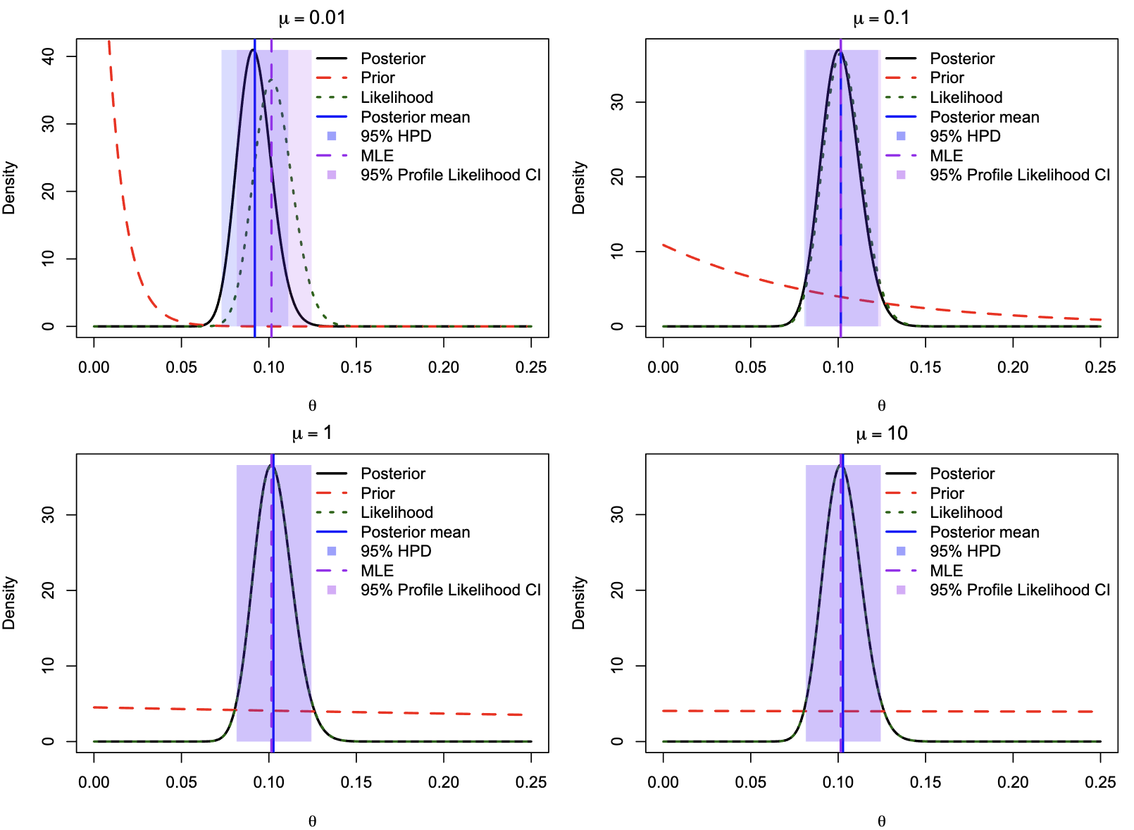
*6.2.3 Classical versus Bayesian Statistics
- 6.2.3.1 Criticisms of Frequentist Statistics (from Bayesian perspective):
- Frequentist methods make probability statements about data or procedures, not directly about parameters of interest after data is observed.
- Confidence Intervals: A 95% CI means that if we repeat the experiment many times, 95% of such constructed intervals will contain the true parameter. It does not mean there’s a 95% probability that the specific interval we calculated contains the true parameter. (Fig 6.4)
- p-values: The probability of observing data as extreme or more extreme than what was actually observed, if the null hypothesis ($H_0$) were true. It is not $P(H_0\vert \text{data})$.
- Likelihood Principle Violation: p-values can depend on the stopping rule of an experiment (e.g., fixed $n$ trials vs. fixed number of successes), even if the likelihood function $L(\theta\vert x)$ is the same. (Fig 6.5 - binomial vs. negative binomial). Bayesian inference respects the likelihood principle.
- 6.2.3.2 Criticisms of Bayesian Methods (from Frequentist perspective):
- Levied on the prior distribution $f(\theta)$.
- Objective Bayes: Aims to represent “prior ignorance.”
- Uniform priors (principle of insufficient reason) seem intuitive for ignorance but lead to contradictions because they are not invariant to parameter transformations (e.g., uniform on side length $a$ vs. uniform on area $A=a^2$).
- No single prior truly represents “total ignorance.”
- Subjective Bayes: Prior represents researcher’s personal belief.
- Classical statisticians reject incorporating personal beliefs into scientific inference.
- Likelihood models also involve subjectivity but can be checked against data; priors often cannot.
- 6.2.3.3 Does it Matter?
- Stable Estimation Problems: Well-formulated model, large dataset. Prior has little effect. Likelihood and Bayesian estimates (and CIs/credibility intervals) are similar. (e.g., Example 6.4, Fig 6.3, Fig 6.6).
- Prior and Likelihood Both Influential: Ill-formulated/barely identifiable models, sparse data. Posterior is sensitive to prior. Classical and Bayesian results may differ.
- Hypothesis Testing/Model Selection with Vague Priors: Bayesian results can be highly sensitive to prior choice.
- Lindley’s Paradox: For $H_0: \mu=0$ vs. $H_1: \mu \ne 0$ (normal data). Large $n$, small $\bar{x}$ can lead to small p-value (reject $H_0$), but Bayesian analysis with a diffuse prior on $\mu$ under $H_1$ can strongly support $H_0$ ($P_0 \approx 1$). (Eq 6.27-6.33)
- This happens because a diffuse prior spreads probability thinly over a wide range, making the marginal likelihood $M_1 = \int L_1(\mu)f(\mu\vert H_1)d\mu$ small.
- The posterior model probability $P_0$ is sensitive to the “diffuseness” (e.g., variance $\sigma_0^2$) of the prior on $\mu$ under $H_1$. (Eq 6.33, 6.36)
6.3 Prior
Specification of the prior distribution $f(\theta)$.
6.3.1 Methods of Prior Specification
- Prior should reflect belief before data analysis. Can use past experiments or model the physical/biological process.
- Vague/Diffuse Priors (Objective Bayes idea): Used when little prior information.
- Principle of insufficient reason (uniform).
- Invariance to reparameterization (Jeffreys prior).
- Maximization of missing information (Reference prior).
- Hierarchical Bayesian Approach: If prior involves unknown parameters (hyper-parameters), assign priors to them (hyper-priors). Usually 2-3 levels.
- Empirical Bayes (EB): Estimate hyper-parameters from the marginal likelihood of the data $f(x\vert \text{hyper-param}) = \int f(\theta\vert \text{hyper-param})f(x\vert \theta)d\theta$, then use these estimates in the prior for $\theta$. Widely used in phylogenetics (e.g., estimating site rates, ASR).
- Robustness Analysis: Always assess sensitivity of posterior to prior choice. If posterior dominated by data, prior choice is less critical.
6.3.2 Conjugate Priors
- Prior and posterior have the same distributional form. Likelihood updates parameters of the distribution.
- Beta prior for binomial $\theta$: Likelihood $\theta^x(1-\theta)^{n-x}$. Prior $\theta^{a-1}(1-\theta)^{b-1}$. Posterior $\theta^{x+a-1}(1-\theta)^{n-x+b-1}$. (Eq 6.37-6.39)
- $U(0,1) \equiv \text{Beta}(1,1)$.
- Jeffreys prior for binomial $\theta$ is $\text{Beta}(1/2, 1/2)$.
- Haldane’s prior $\text{Beta}(0,0)$ (improper, $f(\theta) \propto \theta^{-1}(1-\theta)^{-1}$) gives posterior mean = MLE ($x/n$).
- Gamma prior for Poisson rate $\lambda$: Likelihood $\lambda^{\sum x_i} e^{-n\lambda}$. Prior $\lambda^{\alpha-1}e^{-\beta\lambda}$. Posterior $\lambda^{\sum x_i+\alpha-1}e^{-(n+\beta)\lambda}$. (Eq 6.40-6.43)
- Normal prior for normal mean $\mu$ (known $\sigma^2$): Posterior is also normal. Posterior mean is weighted average of prior mean and sample mean, weights are precisions (inverse variances). Posterior precision = prior precision + sample precision. (Eq 6.44)
- Rarely used in complex phylogenetic models.
- Common when little information.
- Improper Prior: If it doesn’t integrate to 1. Permissible if posterior is proper.
- May not be biologically reasonable (e.g., $U(0,10)$ for JC69 distance $\theta$ implies most distances are large, while data suggests small).
- Can cause MCMC convergence problems.
- For JC69 distance $\theta$, uniform prior on $p$ (proportion of different sites) $p \sim U(0, 3/4)$ implies $f(\theta) = \frac{4}{3}e^{-4\theta/3}$ (Eq 6.47), favoring small distances. This is more reasonable than uniform on $\theta$.
*6.3.4 The Jeffreys Priors
- Based on Fisher information $I(\theta)$. Invariant to reparameterization.
- $f(\theta) \propto [\det I(\theta)]^{1/2}$ (Eq 6.49)
- For binomial $\theta$: $I(\theta) = n/(\theta(1-\theta))$. Prior $f(\theta) \propto \theta^{-1/2}(1-\theta)^{-1/2}$, which is $\text{Beta}(1/2, 1/2)$. (Eq 6.52)
- For JC69 distance $\theta$: $f(\theta) \propto (e^{8\theta/3} + 2e^{4\theta/3} - 3)^{-1/2}$. (Eq 6.56)
- Reference prior is often Jeffreys prior for single parameter models. Rarely used in phylogenetics.
*6.3.5 The Reference Priors
- Maximizes expected K-L divergence between prior and posterior (maximizes missing information in prior).
- Formal procedure for derivation. Jeffreys prior for regular single-parameter models.
- Rarely used in phylogenetics.
6.4 Methods of Integration
Calculating the marginal likelihood $f(X) = \int f(\theta)f(X\vert \theta)d\theta$ is hard, especially for high-dimensional $\theta$.
*6.4.1 Laplace Approximation
- For large sample size $n$, likelihood $L(\theta) = e^{nh(\theta)}$ is highly peaked around MLE $\hat{\theta}$.
- Approximate $h(\theta)$ by Taylor expansion around $\hat{\theta}$: $h(\theta) \approx h(\hat{\theta}) + \frac{1}{2}(\theta-\hat{\theta})^T H (\theta-\hat{\theta})$, where $H = \frac{d^2h}{d\theta^2}\vert _{\hat{\theta}}$.
- $I = \int f(\theta)e^{nh(\theta)}d\theta \approx f(\hat{\theta})L(\hat{\theta}) \sqrt{(2\pi)^p \vert V\vert }$ (Eq 6.66 for multivariate)
where $V = -(nH)^{-1}$ is the asymptotic variance-covariance matrix of $\hat{\theta}$, $p$ is dimension of $\theta$.
For univariate: $I \approx f(\hat{\theta})L(\hat{\theta}) \sqrt{2\pi V}$ (Eq 6.64).
- Relatively accurate for peaked likelihoods.
6.4.2 Mid-point and Trapezoid Methods
- Numerical integration by dividing interval $[a,b]$ into $n$ segments. (Fig 6.7)
- Mid-point: Sum areas of rectangles (height = function value at mid-point of segment). (Eq 6.68)
- Trapezoid: Sum areas of trapezoids. (Eq 6.69)
6.4.3 Gaussian Quadrature
- Approximates $\int_{-1}^1 f(x)dx \approx \sum_{i=1}^N w_i f(x_i)$ using pre-determined points $x_i$ and weights $w_i$. (Eq 6.70)
- Exact if $f(x)$ is a polynomial of degree $2N-1$ or less.
- Integral over $(a,b)$ converted to $(-1,1)$ by linear transform (Eq 6.71).
- Curse of Dimension: For $d$-dimensional integrals, $N^d$ points needed. Feasible for low dimensions (1-3) only.
6.4.4 Marginal Likelihood Calculation for JC69 Distance Estimation
- Illustrates numerical integration for $I = \int_0^\infty f(\theta)f(x\vert \theta)d\theta$ from Example 6.4. (Eq 6.62)
- Requires transforming $\theta \in (0, \infty)$ to $y \in (-1,1)$ or similar finite range. (Table 6.1, Fig 6.8)
- Transform 1: $y = (\theta-1)/(\theta+1)$ (Eq 6.73) $\rightarrow I_1$ (Eq 6.74)
- Transform 2 (based on $p$): $y = \frac{8}{3}p-1$ (Eq 6.75) $\rightarrow I_2$ (Eq 6.76)
- Transform 3 (log-$t_2$ sigmoid): Based on fitting log $\theta$ with a $t_2$ distribution. (Eq 6.79, 6.80)
- Transform 4 (log-logistic sigmoid): Based on fitting log $\theta$ with a logistic distribution. (Eq 6.82, 6.83)
- Results: Quadrature methods (esp. with good transforms like log-$t_2$ or log-logistic) are much more accurate than mid-point/trapezoid for same number of points $N$. Good transforms flatten the integrand.
6.4.5 Monte Carlo (MC) Integration
- To compute $I = E_f[h(\theta)] = \int h(\theta)f(\theta)d\theta$.
- Draw $N$ samples $\theta_i$ from $f(\theta)$. Estimate $\hat{I} = \frac{1}{N}\sum_{i=1}^N h(\theta_i)$. (Eq 6.84, 6.85)
- Variance of $\hat{I}$ depends on $N$, not dimensionality of $\theta$. (Eq 6.86)
- For marginal likelihood $f(X)$, $f(\theta)$ is prior, $h(\theta)$ is likelihood $f(X\vert \theta)$.
- Inefficient if prior $f(\theta)$ is very different from posterior (i.e., if likelihood $h(\theta)$ is sharply peaked and prior is diffuse), as most samples $\theta_i$ will have tiny $h(\theta_i)$. (Table 6.2)
6.4.6 Importance Sampling
- Sample $\theta_i$ from a different proposal distribution $g(\theta)$ instead of $f(\theta)$.
- $I = E_g \left[ h(\theta) \frac{f(\theta)}{g(\theta)} \right]$. Estimate $\hat{I}{IS} = \frac{1}{N}\sum{i=1}^N h(\theta_i) \frac{f(\theta_i)}{g(\theta_i)}$. (Eq 6.87, 6.88)
- $w(\theta_i) = f(\theta_i)/g(\theta_i)$ are importance weights.
- Optimal $g(\theta) \propto h(\theta)f(\theta)$ (i.e., the posterior), but this requires knowing $I$.
- Choose $g(\theta)$ to be similar to posterior, and heavier-tailed than $f(\theta)$.
- Alternative form (sampling from unnormalized $g^$):
$I_{IS}^ = \frac{\sum h(\theta_i) f(\theta_i)/g^(\theta_i)}{\sum f(\theta_i)/g^(\theta_i)}$ (Eq 6.90) (More robust to unbounded $f/g$ ratios).
- Using log-$t_2$ or log-logistic as sampling distributions $g(\theta)$ for JC69 example greatly improves efficiency over simple MC. (Table 6.2)
7. Bayesian computation (MCMC)
This chapter delves into Markov chain Monte Carlo (MCMC) methods, which are simulation algorithms essential for Bayesian computation, particularly when the posterior distribution is complex and cannot be analyzed analytically.
7.1 Markov Chain Monte Carlo
7.1.1 Metropolis Algorithm
- Concept: MCMC generates a dependent sample $(\theta_1, \theta_2, …, \theta_n)$ from a target probability density $\pi(\theta)$ (typically the posterior distribution $f(\theta\vert X)$). This sequence forms a stationary Markov chain whose states are the possible values of $\theta$.
- Estimating Expectations: The expectation of a function $h(\theta)$ over $\pi(\theta)$, which is an integral $I = E_{\pi}{h(\theta)} = \int h(\theta)\pi(\theta) d\theta$ (Eq 7.1), can be estimated by the sample average:
$\tilde{I} = \frac{1}{n} \sum_{i=1}^{n} h(\theta_i)$ (Eq 7.2)
- Variance of the Estimate: Unlike independent Monte Carlo integration, the variance of $\tilde{I}$ from an MCMC sample must account for autocorrelation. If $\rho_k = \text{corr}(h(\theta_i), h(\theta_{i+k}))$ is the autocorrelation at lag $k$:
$\text{var}(\tilde{I}) = \text{var}(\hat{I}) \times [1 + 2(\rho_1 + \rho_2 + \rho_3 + \dots)] = \text{var}(\hat{I}) \times \tau$ (Eq 7.3)
where $\text{var}(\hat{I})$ is the variance for an independent sample, and $\tau = [1 + 2\sum \rho_k]$ is the autocorrelation time.
- Effective Sample Size (ESS): The efficiency of the MCMC sample relative to an independent sample is $E = \text{var}(\hat{I})/\text{var}(\tilde{I}) = 1/\tau$ (Eq 7.4). An MCMC sample of size $n$ is as informative as an independent sample of size $nE = n/\tau$.
- Why MCMC? It’s often hard to generate independent samples from the posterior, but MCMC provides a way to generate dependent samples.
Metropolis Algorithm (Metropolis et al., 1953) - Illustrated with a 3-state discrete example (robot on boxes, Fig 7.1a):
Let $\theta$ take values ${1, 2, 3}$ with target probabilities $\pi_1, \pi_2, \pi_3$.
- Initialization: Set initial state (e.g., $\theta = 1$).
- Proposal: Propose a new state $\theta’$ from the current state $\theta$. In this simple symmetric example, choose one of the two alternative states with probability $1/2$ each.
- Accept/Reject:
- If $\pi(\theta’) > \pi(\theta)$, accept $\theta’$ (move to the higher box).
- Otherwise (if $\pi(\theta’) \le \pi(\theta)$), accept $\theta’$ with probability $\alpha = \frac{\pi(\theta’)}{\pi(\theta)}$.
- If the proposal is accepted, the next state is $\theta’$. Otherwise, the next state remains $\theta$.
(This can be implemented by drawing $u \sim U(0,1)$; if $u < \alpha$, accept, else reject).
- Record: Print out the current state.
- Iterate: Go to step 2.
Key Features of Metropolis Algorithm:
- Ratio of Densities: Only the ratio $\frac{\pi(\theta’)}{\pi(\theta)}$ is needed, not $\pi(\theta)$ itself. This is crucial because for posteriors, $\pi(\theta) = f(\theta\vert X) = \frac{f(\theta)f(X\vert \theta)}{f(X)}$. The normalizing constant $f(X)$ (marginal likelihood) is often very hard to compute but cancels out in the ratio:
$\alpha = \min\left(1, \frac{\pi(\theta’)}{\pi(\theta)}\right) = \min\left(1, \frac{f(\theta’)f(X\vert \theta’)}{f(\theta)f(X\vert \theta)}\right)$ (Eq 7.5)
This allows sampling from the posterior without calculating $f(X)$.
- Markov Chain: The sequence of states is a Markov chain (next state depends only on current state).
- Stationary Distribution: If run long enough, the proportion of time spent in each state $i$ will be $\pi_i$. So, $\pi(\theta)$ is the stationary distribution of the chain.
- Proof Sketch (Detailed Balance): The net flow from state $i$ to state $j$ is $f_i P_{ij} - f_j P_{ji}$. If $\pi_i \le \pi_j$, then $P_{ij}$ (proposal $i \to j$) is $1 \times \text{Prob(propose j from i)}$, and $P_{ji}$ is $\frac{\pi_i}{\pi_j} \times \text{Prob(propose i from j)}$. For symmetric proposals, $\text{Prob(propose j from i)} = \text{Prob(propose i from j)}$. The net flow is proportional to $f_i - f_j \frac{\pi_i}{\pi_j}$. This flow is positive (from $i$ to $j$) if $f_i/f_j > \pi_i/\pi_j$, meaning state $i$ is currently overrepresented relative to $j$. The chain moves to correct this imbalance, eventually reaching $f_i/f_j = \pi_i/\pi_j$. The chain is reversible under detailed balance.
- Continuous Parameters: The algorithm is essentially the same.
- Example 7.1 (JC69 distance $\theta$):
- Prior: $f(\theta) = \frac{1}{\mu} e^{-\theta/\mu}$
- Likelihood: $f(x\vert \theta) = \left(\frac{3}{4} - \frac{3}{4}e^{-4\theta/3}\right)^x \left(\frac{1}{4} + \frac{3}{4}e^{-4\theta/3}\right)^{n-x}$ (Eq 7.6)
- Proposal: Sliding window $\theta’ \sim U(\theta - w/2, \theta + w/2)$. If $\theta’<0$, reflect ($\theta’ = -\theta’$).
- Acceptance ratio $\alpha$: As in Eq 7.7 (using product of prior ratio and likelihood ratio).
- Window Size ($w$): Critical for mixing. (Fig 7.2a)
- Too small $w$: High acceptance ($P_{jump}$), but tiny steps (poor mixing, high autocorrelation).
- Too large $w$: Low acceptance ($P_{jump}$), chain gets stuck (poor mixing).
- Optimal $P_{jump}$ often around 20-50% (e.g., ~30-40% for normal-like 1D targets).
- Burn-in: Initial samples are discarded until the chain reaches stationarity (Fig 7.2b).
- Posterior can be summarized by histogram (Fig 7.2c) or kernel density estimate (Fig 7.2d).
7.1.2 Asymmetrical Moves and Proposal Ratio (Metropolis-Hastings)
- Metropolis-Hastings (MH) Algorithm (Hastings, 1970): Generalizes Metropolis to allow asymmetric proposal densities $q(\theta’\vert \theta)$ (probability of proposing $\theta’$ given current $\theta$).
- Acceptance Ratio $\alpha$ modified:
$\alpha(\theta, \theta’) = \min \left(1, \frac{\pi(\theta’)}{\pi(\theta)} \times \frac{q(\theta\vert \theta’)}{q(\theta’\vert \theta)}\right)$
$= \min \left(1, \text{prior ratio} \times \text{likelihood ratio} \times \text{proposal ratio} \right)$ (Eq 7.8)
The term $\frac{q(\theta\vert \theta’)}{q(\theta’\vert \theta)}$ is the Hastings ratio or proposal ratio, correcting for asymmetry in proposals.
- Robot Example (Fig 7.1b): Robot has ‘left bias’ (proposes left box with $2/3$, right with $1/3$).
- If current $\theta=1$, propose $\theta’=2$. $q(2\vert 1) = 1/3$ (assuming it picks right with $1/3$). For reverse move, if current $\theta=2$, propose $\theta’=1$. $q(1\vert 2) = 2/3$ (assuming it picks left with $2/3$).
- Proposal ratio $q(1\vert 2)/q(2\vert 1) = (2/3)/(1/3) = 2$.
- Conditions for Convergence: Proposal density $q(\cdot\vert \cdot)$ must define an irreducible (can reach any state from any state) and aperiodic (no fixed cycles) chain.
7.1.3 The Transition Kernel
- For a continuous state space, the Markov chain is defined by a transition kernel $p(x, y)$, the probability density of moving to state $y$ given current state $x$.
- For MH:
$p(x, y) = q(y\vert x) \cdot \alpha(x, y)$, for $y \neq x$
$p(x, x) = 1 - \int q(y\vert x) \cdot \alpha(x, y) dy$ (probability of rejection, staying at $x$) (Eq 7.9, 7.10, 7.11)
- There’s typically a point mass at $y=x$ due to rejections.
- Acceptance Proportion ($P_{jump}$): Overall probability that a proposal is accepted.
$P_{jump} = \iint \pi(x) q(y\vert x) \alpha(x, y) dx dy = \int \pi(x) (1 - p(x,x)) dx$ (Eq 7.12)
7.1.4 Single-Component Metropolis-Hastings Algorithm
- For multi-parameter models $\theta = (x, y, z, \dots)$, updating all parameters simultaneously can be difficult or inefficient.
- Single-Component MH: Update parameters (or blocks of parameters) one at a time, conditioning on the current values of other parameters.
- Iteration (3 blocks $x,y,z$):
- Propose $x^{\ast}$ from $q(x^{\ast} \vert x, y, z)$. Accept with probability $\alpha_x$ based on $\frac{\pi(x^{\ast}, y, z)}{\pi(x, y, z)}$ and proposal ratio for $x$. Update $x \to x’$.
- Propose $y^{\ast}$ from $q(y^{\ast} \vert x’, y, z)$. Accept with probability $\alpha_y$ based on $\frac{\pi(x’, y^{\ast}, z)}{\pi(x’, y, z)}$ and proposal ratio for $y$. Update $y \to y’$.
- Propose $z^{\ast}$ from $q(z^{\ast} \vert x’, y’, z)$. Accept with probability $\alpha_z$ based on $\frac{\pi(x’, y’, z^{\ast})}{\pi(x’, y’, z)}$ and proposal ratio for $z$. Update $z \to z’’$.
- The ratio of joint posteriors simplifies to the ratio of full conditional distributions. For step 2:
$\frac{\pi(x’, y^{\ast}, z)}{\pi(x’, y, z)} = \frac{\pi(y^{\ast} \vert x’, z)}{\pi(y \vert x’, z)}$ (Eq 7.16)
- Allows tailoring proposal mechanisms for different components. Advisable to block highly correlated parameters and update them together.
7.1.5 Gibbs Sampler
- A special case of single-component MH.
- To update a component (e.g., $y$), propose directly from its full conditional distribution: $q(y^{\ast} \vert x’, y, z) = \pi(y^{\ast} \vert x’, z)$.
- This makes the acceptance ratio $\alpha = 1$ always (Eq 7.13-7.16). All proposals are accepted.
- Widely used in linear models where priors and likelihoods are normal, making full conditionals also normal and easy to sample from.
- Seldom used in phylogenetics as full conditionals are usually complex.
7.2 Simple Moves and Their Proposal Ratios
The proposal ratio depends only on the proposal algorithm, not the prior or likelihood.
- 7.2.1 Sliding Window with Uniform Proposal:
- $x’ \sim U(x - w/2, x + w/2)$ (Eq 7.17)
- Proposal ratio is 1 because $q(x’\vert x) = q(x\vert x’) = 1/w$.
- Constraints: If $x \in (a,b)$, reflections are used for proposed values outside the interval. E.g., if $x’ < a$, new $x’ = a + (a-x’) = 2a-x’$.
- Proposal ratio remains 1 even with reflections.
- 7.2.2 Sliding Window with Normal Proposal:
- $x’\vert x \sim N(x, \sigma^2)$ (Eq 7.18)
- Proposal ratio is 1 because $q(x’\vert x) = q(x\vert x’)$. (Normal PDF is symmetric around mean).
- Handles constraints by reflection, proposal ratio still 1.
- 7.2.3 Bactrian Proposal (Yang & Rodriguez 2013):
- Aims to avoid proposing states very close to current state. Shaped like a two-humped camel.
- Standard Bactrian: 1:1 mixture of $N(-m, 1-m^2)$ and $N(m, 1-m^2)$. Mean 0, variance 1. Parameter $m \in [0,1)$ controls “spikiness”.
- To use as sliding window: $x’ = x + y\sigma$, where $y$ is from standard Bactrian, $\sigma$ is step size.
- Proposal density $q(x’\vert x; m, \sigma^2) = \frac{1}{2\sigma\sqrt{1-m^2}} \left[ \exp\left(-\frac{(x’-x+m\sigma)^2}{2\sigma^2(1-m^2)}\right) + \exp\left(-\frac{(x’-x-m\sigma)^2}{2\sigma^2(1-m^2)}\right) \right]$ (Eq 7.20)
- Symmetric, so proposal ratio is 1. Often more efficient than uniform/normal. $m=0.95$ is a good choice. (Fig 7.4)
- 7.2.4 Sliding Window with Multivariate Normal Proposal:
- To update $k$ parameters $x = (x_1, …, x_k)$ at once.
- Simplest: $x’\vert x \sim N_k(x, I\sigma^2)$ where $I$ is identity matrix. Proposal ratio 1.
- Inefficient if parameters have different scales or are correlated (Fig 7.5).
- Better: $x’\vert x \sim N_k(x, S\sigma^2)$, where $S$ is an estimate of the posterior variance-covariance matrix. (Can be estimated from pilot runs). This accounts for scales and correlations. Proposal ratio is still 1.
- 7.2.5 Proportional Scaling (Multiplier Proposal):
- Useful for positive parameters (e.g., branch lengths, rates).
- $x’ = x \cdot c$, where $c = e^{\lambda(u-1/2)}$ and $u \sim U(0,1)$. $\lambda$ is a tuning parameter.
- Proposal density (from variable transform): $q(x’\vert x) = 1/(\lambda\vert x’\vert )$ (Eq 7.22, assuming $x’>0$).
- Proposal ratio: $q(x\vert x’)/q(x’\vert x) = \vert x’\vert /\vert x\vert = c$.
- Alternative view: it’s a sliding window on $y = \log(x)$, where $y’ \sim U(y-\lambda/2, y+\lambda/2)$. Jacobian of transform $\log(x) \to x$ is $e^y=x$. Proposal ratio from Theorem 2 (Appendix A) is $x’/x = c$.
- Cannot move a parameter from 0. Bounds handled by reflection in log-space.
- Can scale multiple parameters $x_i’ = c x_i$. Proposal ratio is $c^m$ for $m$ parameters.
- 7.2.6 Proportional Scaling with Bounds:
- For $m$ variables $x_i \in (a,b)$.
- Transform: $y_i = (b-x_i)/(x_i-a)$, so $y_i \in (0, \infty)$. (Eq 7.23)
- Apply proportional scaling to $y_i$: $y_i’ = y_i \cdot c$. (Eq 7.24)
- Proposal ratio for $x$: $c^m \times \prod_{i=1}^m \left(\frac{x_i’-a}{x_i-a}\right)^2$. (Eq 7.26)
7.3 Convergence, Mixing, and Summary of MCMC
7.3.1 Convergence and Tail Behaviour
- 7.3.1.1 Rejection Rate and Light/Heavy Tails:
- Geometric Convergence: Distance between current distribution and stationary distribution $\pi(x)$ decreases by $r^n$ ($r<1$) in $n$ steps.
- Mengersen & Tweedie (1996): For 1D MCMC, geometric convergence if and only if $\lim_{x\to\infty} \nabla \log \pi(x) < 0$. (Eq 7.27)
- This means the posterior must be light-tailed (e.g., normal, exponential, gamma).
- Heavy-tailed posteriors (e.g., Cauchy, t-dist, inverse gamma) may lead to non-geometric convergence (random walk behavior in tails).
- Tail Paradox: For light-tailed posteriors, the further in the tail, the flatter $\pi(x)$ is, but the steeper $\nabla \log \pi(x)$ is, leading to faster movement out of the tail. (Example: Normal distribution, Eq 7.28).
- For heavy-tailed posteriors (e.g., inverse gamma, Eq 7.29), $\nabla \log \pi(x) \to 0$, so acceptance ratio for moves to right approaches 1. Chain behaves like random walk, very slow convergence if started in tail.
- Multidimensional Problem: (Roberts & Tweedie, 1996) Posterior must be light-tailed AND “smooth” (no sharp ridges) (Fig 7.6 example, Eq 7.30).
- 7.3.1.2 Multiple Modes in the Posterior:
- Can cause serious convergence/mixing problems if MCMC gets trapped in a local mode.
- Often due to conflict between prior and likelihood (Fig 7.7, 7.8).
- Example: Human-chimp 12S rRNA distance. Informative (unreasonable) gamma prior $G(100,10)$ (mean 10, var 1) conflicts with likelihood (MLE $\approx 0.01172$). Posterior has two modes, one near MLE, one near prior mean (Fig 7.8). MCMC might get stuck in the very low prior-induced mode if started there.
7.3.2 Mixing Efficiency, Jump Probability, and Step Length
Focus on discrete state chains first for theory, then continuous.
- 7.3.2.1 Discrete State Chains:
- Asymptotic variance of $\tilde{I} = \frac{1}{n}\sum h(X_i)$ can be calculated from transition matrix $P={p_{ij}}$ (Eq 7.35, 7.37). $v = h^T B (2Z - I - A) h$, where $Z = [I-(P-A)]^{-1}$ is fundamental matrix.
- Efficiency related to second largest eigenvalue $\lambda_2$ of $P$. Smaller $\vert \lambda_2\vert $ means better mixing.
- Peskun’s Theorem (1973): For two reversible chains $P^{(1)}, P^{(2)}$ with same stationary $\pi$, if $p^{(1)}{ij} \ge p^{(2)}{ij}$ for all $i \ne j$ (i.e., $P^{(1)}$ has larger off-diagonal elements), then $P^{(1)}$ is more efficient (smaller variance for estimates of $I$). More mobile chains are better.
- Two States: Optimal $p_{12} = \pi_2/\pi_1$ and $p_{21}=1$ (if $\pi_1 \ge \pi_2$). Efficiency $E = p_{12}/(2\pi_2 - p_{12})$. (Eq 7.40)
- K States: Highest $P_{jump} = 2(1-\pi_1)$ (if states ordered by $\pi_i$). (Eq 7.41, 7.42).
- Frigessi et al. (1992) construction for P achieving optimal $\lambda_2 = -\pi_K/(1-\pi_K)$. (Eq 7.43-7.46).
- 7.3.2.2 Efficiency of Continuous State Chains:
- Discretize state space to use discrete theory.
- Gelman et al. (1996): For $N(0,1)$ target and $N(x, \sigma^2)$ proposal, optimal $\sigma \approx 2.5$ (relative to target SD), gives $P_{jump} \approx 0.43$, efficiency $E \approx 0.23$. (Table 7.2)
- Yang & Rodriguez (2013): Compared proposals for different targets (Fig 7.9, 7.10, Table 7.2).
- Bactrian proposal generally best, then uniform, then normal.
- Bactrian with $m=0.95$ often optimal, $P_{jump} \approx 0.3$.
- 7.3.2.3 Convergence Rate and Step Length:
- Convergence rate dominated by $R = \max_{k\ge 2} \vert \lambda_k\vert $.
- Optimal step length for fast convergence can be slightly larger than for efficient mixing (for uniform/normal). Suggests larger steps in burn-in.
- 7.3.2.4 Automatic Adjustment of Step Length:
- $P_{jump}$ is usually monotonic with step length $\sigma$. Can adjust $\sigma$ during burn-in to achieve target $P_{jump}$ (e.g., 0.3-0.4).
- For Normal target & Normal proposal: $P_{jump} = \frac{2}{\pi} \tan^{-1}(\sigma/2)$. Can invert to find optimal $\sigma^*$ given current $\sigma, P_{jump}$ (Eq 7.50, 7.51, Fig 7.12, 7.13).
- Similar logic can be applied for Bactrian, though integral for $P_{jump}$ is more complex (Eq 7.52).
7.3.3 Validating and Diagnosing MCMC Algorithms
- MCMC enables complex models but introduces computational challenges (correctness, convergence, mixing).
- Diagnostic Strategies:
- Time-series (Trace) Plots: Plot parameter values against iteration number. Look for stability, good exploration.
- Acceptance Proportion: Should be in a reasonable range (e.g., 20-50% for many proposals).
- Multiple Chains: Run from different, over-dispersed starting points. Should converge to same distribution.
- Run with No Data: Posterior should equal prior.
- Simulate Data: Analyze simulated data (where truth is known) to see if Bayesian estimates are consistent and CIs have correct coverage.
- Hit Probability: Proportion of CIs that include the true parameter value.
- Coverage Probability: Average posterior probability density within a fixed prior interval.
7.3.4 Potential Scale Reduction Statistic ($\hat{R}$)
- Gelman & Rubin (1992): Uses multiple chains ($m$) of length $n$ (post burn-in).
- Compares within-chain variance ($W$) and between-chain variance ($B$).
- $B = \frac{n}{m-1} \sum_{i=1}^m (\bar{x}{i\cdot} - \bar{x}{\cdot\cdot})^2$ (Eq 7.53)
- $W = \frac{1}{m(n-1)} \sum_{i=1}^m \sum_{j=1}^n (x_{ij} - \bar{x}_{i\cdot})^2$ (Eq 7.54)
- Estimate of posterior variance: $\hat{\sigma}^2 = \frac{n-1}{n}W + \frac{1}{n}B$ (Eq 7.55)
- Potential Scale Reduction Factor: $\hat{R} = \sqrt{\hat{\sigma}^2 / W}$ (Eq 7.56)
- $\hat{R}$ approaches 1 as chains converge. Values $< 1.1$ or $< 1.2$ often indicate convergence.
7.3.5 Summary of MCMC Output
- Burn-in: Discard initial samples.
- Thinning: Sample every $k^{th}$ iteration to reduce autocorrelation and file size (though theoretically less efficient than using all samples).
- Marginal Posterior: For a parameter $\theta$, use its samples, ignoring others. Visualize with histogram/density plot.
- Point Estimate: Sample mean or median.
- Credible Interval (CI):
- Equal-tail CI: e.g., 2.5% and 97.5% percentiles of sorted samples.
- Highest Posterior Density (HPD) Interval: Shortest interval containing (e.g.) 95% of posterior mass. For unimodal, can be found by finding shortest interval among $((j), (j+0.95n))$ from sorted samples (Fig 7.14). More complex for multimodal.
- Autocorrelation Time ($\tau$) / ESS ($n/\tau$): Can be estimated from output using methods like initial positive sequence (Geyer 1992).
7.4 Advanced Monte Carlo Methods
This section discusses MCMC algorithms designed to handle more challenging situations, such as posteriors with multiple local peaks or the need to compare models of different dimensions.
7.4.1 Parallel Tempering (MC³)
- Problem: Standard MCMC can get stuck in local peaks of a rugged posterior distribution (Fig 7.15).
- Metropolis-Coupled MCMC (MC³ or MCMCMC): (Geyer 1991; Marinari & Parisi 1992).
- Run $m$ Markov chains in parallel.
- Each chain $j$ samples from a “heated” (flattened) version of the target posterior $\pi(\theta)$:
$\pi_j(\theta) \propto [\pi(\theta)]^{1/T_j}$ (Eq 7.57)
where $T_j$ is the “temperature” for chain $j$.
- Typically, $T_j = 1 + \delta(j-1)$ with $\delta > 0$.
- The first chain ($j=1, T_1=1$) is the cold chain and samples from the true posterior $\pi(\theta)$. This is the chain used for inference.
- Other chains ($j>1, T_j > 1$) are hot chains. Higher $T_j$ means a flatter surface, allowing these chains to cross valleys between peaks more easily.
- Within-chain moves: Each chain $j$ performs standard MH updates using its target $\pi_j(\theta)$. Acceptance for a symmetric move from $\theta$ to $\theta’$ in chain $j$:
$\alpha = \min \left(1, \left[\frac{\pi(\theta’)}{\pi(\theta)}\right]^{1/T_j}\right)$ (Eq 7.58)
- Chain Swaps: Periodically, attempt to swap the current states $(\theta_i, \theta_j)$ between two randomly chosen chains $i$ and $j$. The acceptance probability for swapping states:
$\alpha_{swap} = \min \left(1, \frac{\pi_i(\theta_j)}{\pi_i(\theta_i)} \times \frac{\pi_j(\theta_i)}{\pi_j(\theta_j)}\right) = \min \left(1, \left[\frac{\pi(\theta_j)}{\pi(\theta_i)}\right]^{1/T_i - 1/T_j}\right)$ (Eq 7.59)
Swapping allows the cold chain to occasionally receive a state from a hot chain that might have explored a different peak.
- Optimal Temperature Spacing: Atchadé et al. (2011) suggest spacing temperatures so that ~23.4% of chain swaps are accepted.
- Drawback: Only the cold chain’s output is used for inference, making it computationally more expensive as $m-1$ chains are run primarily to improve mixing of the cold chain.
- Widely used in phylogenetics (e.g., MrBayes).
- Fig 7.16 shows how a standard MCMC gets stuck in one of three peaks, while MC³ aims to allow transitions between them.
7.4.2 Trans-model and Trans-dimensional MCMC
Used when comparing different models or models with different numbers of parameters.
7.4.2.1 General Framework
- Goal: Sample from the joint posterior of model indicator $H_k$ and its parameters $\theta_k$:
$f(H_k, \theta_k \vert X) = \frac{1}{Z} \pi_k f(\theta_k\vert H_k) f(X\vert H_k, \theta_k)$ (Eq 7.60)
where $Z$ is the normalizing constant (sum of marginal likelihoods over all models, Eq 7.61), $\pi_k$ is prior on model $H_k$.
Can be written as: $f(H_k, \theta_k \vert X) = f(H_k\vert X) f(\theta_k\vert H_k, X)$ (Eq 7.62) (Posterior model prob $\times$ within-model parameter posterior).
7.4.2.2 Trans-model MCMC (Models with Same Number of Parameters)
- If different models $H_1, H_2, …$ have parameters that can be matched up (e.g., $\mu_1 \leftrightarrow \mu_2$, $\sigma_1 \leftrightarrow \sigma_2$).
- The MCMC state is $(k, \theta_k)$. Moves can be within-model (update $\theta_k$ given $H_k$) or between-model (jump from $H_k$ to $H_{k’}$).
- Example (Normal vs. Gamma model for 5 data points, Table 7.3, 7.4):
- $H_1$: Normal $N(\mu, \sigma^2)$, parameters $\theta_1 = (\mu, \sigma)$.
- $H_2$: Gamma $G(\alpha, \beta)$, parameters $\theta_2 = (\alpha, \beta)$.
- Algorithm 1 (Simple Matching): $\mu \leftrightarrow \alpha$, $\sigma \leftrightarrow \beta$.
- Initial model and parameters.
- Within-model move (e.g., update $\mu, \sigma$ if current model is $H_1$).
- Trans-model move (with some probability):
If in $H_1$ (current params $\mu, \sigma$), propose $H_2$ with params $\alpha’=\mu, \beta’=\sigma$.
If in $H_2$ (current params $\alpha, \beta$), propose $H_1$ with params $\mu’=\alpha, \sigma’=\beta$.
Acceptance ratio $\alpha_{1 \leftrightarrow 2} = \min \left(1, \frac{f(H_{new}, \theta_{new}\vert X)}{f(H_{old}, \theta_{old}\vert X)}\right)$. (Eq 7.71)
Proposal ratio is 1 as no new random variables are generated for the parameters.
- Algorithm 2 (Moment Matching): Match means and variances.
To move $H_1 \to H_2$: set $\alpha’ = (\mu/\sigma)^2$, $\beta’ = \mu/\sigma^2$ (so gamma mean is $\mu$, variance is $\sigma^2$).
To move $H_2 \to H_1$: set $\mu’ = \alpha/\beta$, $\sigma’ = \sqrt{\alpha}/\beta$.
The acceptance ratio now includes a Jacobian determinant for the parameter transformation (Eq 7.73, 7.74, 7.75).
- Algorithm 3 (Random Proposal): To move $H_1 \to H_2$, propose new $\alpha’, \beta’$ from distributions centered on current $\mu, \sigma$ (e.g., $\text{new mean } u_1 \sim G(10, 10/\mu)$, $\text{new SD } u_2 \sim G(10, 10/\sigma)$, then set $\alpha’=(u_1/u_2)^2, \beta’=u_1/u_2^2$).
The acceptance ratio includes ratio of proposal densities $g(v_1,v_2)/g(u_1,u_2)$ and the Jacobian (Eq 7.79, 7.80, 7.81).
- Performance: Moment matching (Alg 2) had highest acceptance (70.3%) and efficiency. Simple matching (Alg 1) was very poor (1.1% acceptance).
7.4.2.3 Trans-dimensional MCMC (rjMCMC) (Green 1995)
- For comparing models with different numbers of parameters (different dimensions).
- E.g., $H_1$ with parameter $\theta_1$ (dimension $d_1$) vs. $H_2$ with $\theta_2$ (dimension $d_2$, where $d_1 < d_2$).
- Dimension Matching: To move $H_1 \to H_2$, generate $d_2-d_1$ random auxiliary variables $u \sim g(u)$. Transform $(\theta_1, u) \to \theta_2$ using a deterministic, invertible function $T$. So, $\theta_2 = T(\theta_1, u)$.
- To move $H_2 \to H_1$, use inverse transform $(\theta_1, u) = T^{-1}(\theta_2)$. Drop $u$.
- Acceptance Ratio (e.g., $H_1 \to H_2$):
$R_{12} = \frac{f(H_2)f(\theta_2\vert H_2)f(X\vert H_2, \theta_2)}{f(H_1)f(\theta_1\vert H_1)f(X\vert H_1, \theta_1)} \times \frac{r_{21}}{r_{12}} \times \frac{1}{g(u)} \times \left\vert \frac{\partial \theta_2}{\partial(\theta_1, u)} \right\vert $ (Eq 7.83)
where $r_{12}, r_{21}$ are probabilities of attempting the jump between models, and the last term is the Jacobian.
- Example (JC69 vs K80 for 2 sequences):
- $H_1$ (JC69): param $\theta_1 = (d)$. $H_2$ (K80): params $\theta_2 = (d, \kappa)$. $d_1=1, d_2=2$.
- Auxiliary variable $u = \kappa$. To move $H_1 \to H_2$: keep $d$ same, generate $\kappa \sim g(\kappa)$ (e.g., from its prior).
- To move $H_2 \to H_1$: keep $d$ same, drop $\kappa$.
- Table 7.5 shows different rjMCMC proposals. Algorithm 1 (generating $\kappa$ from prior) most efficient.
- Mixing Problems of rjMCMC:
- Often severe, especially if data is informative (within-model posteriors are concentrated).
- Proposals for new model parameters are often poor, leading to high rejection rates.
- No direct analogue to step-size tuning of within-model MCMC.
- Product-space method (Carlin & Chib 1995) is an alternative but may be difficult for high-dimensional phylogenetic problems.
7.4.2.5 Model Averaging
- If interested in a quantity $\theta$ present in all models, its posterior can be estimated by averaging over models, weighted by posterior model probabilities $f(H_k\vert X)$:
$f(\theta\vert X) = \sum_{k=1}^K f(H_k\vert X) f(\theta\vert H_k, X)$ (Eq 7.89)
- Can be done by sampling $\theta$ from the rjMCMC output irrespective of current model.
- Usefulness:
- Appealing for accounting for model uncertainty.
- If one model strongly dominates ($f(H_k\vert X) \approx 1$), model averaging gives similar result to using best model.
- If several models fit nearly equally well but give different inferences for $\theta$, model averaging is most useful (posterior for $\theta$ might become multimodal).
- If all models fit poorly, model averaging is unlikely to help.
7.4.3 Bayes Factor and Marginal Likelihood
- Bayes Factor ($B_{01}$): Ratio of posterior odds to prior odds for two models $H_0, H_1$. Equals ratio of marginal likelihoods.
$B_{01} = \frac{M_0}{M_1} = \frac{f(X\vert H_0)}{f(X\vert H_1)} = \frac{\int f(X\vert \theta_0, H_0)f(\theta_0\vert H_0)d\theta_0}{\int f(X\vert \theta_1, H_1)f(\theta_1\vert H_1)d\theta_1}$ (Eq 7.91)
- $\text{Posterior Odds} = \text{Prior Odds} \times B_{01}$ (Eq 7.92)
- If prior odds are 1 ($f(H_0)=f(H_1)=1/2$), then $f(H_0\vert X) = B_{01} / (1+B_{01}) = 1/(1+1/B_{01})$ (Eq 7.93)
- Interpretation of $B_{01}$ (Table 7.6).
- Differences from LRT:
- Bayes factor averages over parameters (via prior), LRT optimizes. Priors have strong influence.
- Numerical results differ. Bayes factor (model selection) is often more conservative than LRT (hypothesis testing), less likely to reject $H_0$ for large datasets.
- Bayes factors easily compare non-nested models or >2 models.
- Requires proper priors (marginal likelihood infinite for improper priors if likelihood doesn’t go to zero fast enough).
- Methods for Calculating Marginal Likelihood ($z=f(X)$):
- Arithmetic Mean (Prior): $z \approx \frac{1}{n} \sum f(X\vert \theta_i)$, where $\theta_i \sim f(\theta)$. Inefficient as prior $f(\theta)$ usually far from posterior. (Eq 7.94, 7.95)
- Harmonic Mean (Posterior): $z \approx n / (\sum [1/f(X\vert \theta_i)])$, where $\theta_i \sim f(\theta\vert X)$. Unstable, infinite variance, positive bias. Generally unusable. (Eq 7.96)
- Thermodynamic Integration (Path Sampling): (Lartillot & Philippe 2006)
- Define power posterior $p_\beta(\theta) \propto [f(X\vert \theta)]^\beta f(\theta)$. ($z_\beta$ is its normalizing constant).
- $\log z_1 - \log z_0 = \log f(X) = \int_0^1 E_\beta[\log f(X\vert \theta)] d\beta$ (Eq 7.99-7.101)
- Run MCMC for several $\beta$ values between 0 (prior) and 1 (posterior). Estimate $E_\beta[\log f(X\vert \theta)]$ from each. Numerically integrate.
- Stepping Stone Sampling (Xie et al. 2011):
- $z_1/z_0 = \prod_{k=1}^K (z_{\beta_k}/z_{\beta_{k-1}})$, where $0=\beta_0 < \beta_1 < \dots < \beta_K=1$.
- Each ratio $r_k = z_{\beta_k}/z_{\beta_{k-1}}$ estimated by importance sampling using samples from $p_{\beta_{k-1}}(\theta)$:
$\hat{r}k = \frac{1}{n} \sum{i=1}^n [f(X\vert \theta_i)]^{\beta_k - \beta_{k-1}}$ (Eq 7.104)
- Requires $K-1$ MCMC runs (if prior can be sampled directly).
8. Bayesian phylogenetics
This chapter provides an overview of Bayesian inference as applied to phylogenetic reconstruction, including historical background, MCMC algorithms, model and prior choices, and issues related to interpreting posterior probabilities.
8.1 Overview
8.1.1 Historical Background
- Early Efforts (1960s): Edwards and Cavalli-Sforza attempted to apply Fisher’s likelihood method to infer human population trees using gene frequency data.
- They used the Yule process (pure birth process) for tree probabilities (prior on labeled histories) and Brownian motion for gene frequency drift.
- This work led to the development of distance (additive-tree) and parsimony (minimum-evolution) methods as approximations to ML.
- Edwards (1970) clarified that the tree (or labeled history) should be estimated from its conditional distribution given the data (i.e., the posterior), marking an early application of Bayesian ideas to phylogenetics.
- Introduction to Molecular Phylogenetics (1990s): Three groups independently introduced Bayesian inference for sequence data:
- Rannala and Yang (1996; Yang and Rannala 1997)
- Mau and Newton (1997)
- Li et al. (2000)
- Early studies often assumed a molecular clock and uniform priors on rooted trees (either labeled histories or simple rooted trees).
- Development of MCMC Software:
- BAMBE (Larget and Simon 1999) and MrBayes (Huelsenbeck and Ronquist 2001) implemented more efficient MCMC algorithms.
- The clock constraint was relaxed, allowing for more realistic evolutionary models.
- Tree perturbation algorithms (NNI, SPR, TBR) were adapted as MCMC proposals.
- Later versions of MrBayes (Ronquist et al. 2003, 2012b) incorporated many ML models and can handle heterogeneous multi-gene datasets.
- Modern Bayesian Programs:
- BEAST (Drummond et al. 2006; Drummond and Rambaut 2007): Focuses on estimating rooted trees under clock and relaxed-clock models, particularly for divergence time estimation.
- PhyloBayes (Lartillot et al. 2007, 2009; Lartillot and Philippe 2008): Implements sophisticated models for substitution heterogeneity (e.g., CAT model) important for deep phylogenies.
- These are now standard tools alongside fast ML programs like RAxML and PhyML.
8.1.2 A Sketch MCMC Algorithm
- General Framework:
- Data: Sequence alignment $X$.
- Tree Topology: $\tau_i$, $i=1, \dots, T_s$. Prior $f(\tau_i)$ (often uniform $1/T_s$).
- Branch Lengths: Vector $t_i$ for tree $\tau_i$. Prior $f(t_i \vert \tau_i)$ (often simplified to $f(t_i)$).
- Substitution Model Parameters: $\theta$. Prior $f(\theta)$.
- Joint Posterior Distribution:
$f(\tau_i, t_i, \theta \vert X) \propto f(\theta) f(\tau_i) f(t_i \vert \tau_i) f(X \vert \theta, \tau_i, t_i)$ (Eq 8.1)
The normalizing constant $f(X)$ (marginal likelihood of data) is usually intractable. MCMC avoids its direct calculation.
- Sketch of an MCMC Algorithm:
- Initialization: Start with a random tree $\tau$, random branch lengths $t$, and random substitution parameters $\theta$.
- Iteration: Repeat the following steps:
a. Propose a change to the tree topology $\tau \to \tau’$ (using NNI, SPR, TBR). This may also change branch lengths $t \to t’$.
b. Propose changes to branch lengths $t \to t’$.
c. Propose changes to substitution parameters $\theta \to \theta’$.
d. Every $k$ iterations (thinning), sample the current state $(\tau, t, \theta)$ and save it to disk.
- Summarization: After a sufficient number of iterations (post burn-in), summarize the collected samples.
8.1.3 The Statistical Nature of Phylogeny Estimation
- Tree as a Model: A phylogenetic tree is a statistical model, not just a parameter. Phylogeny reconstruction is therefore a model selection problem.
- Importance of Distinction:
- Asymptotic Efficiency of MLEs: Applies to parameter estimation within a fixed model (e.g., branch lengths on a given tree), not to ML tree topology selection (see §5.2.3).
- MCMC Design: Proposals changing tree topology are cross-model moves and should be designed/optimized differently from within-model moves (parameter changes on a fixed tree).
- Phylogeny vs. Typical Model Selection/Hypothesis Testing:
- Phylogenetics involves a vast number of tree models with complex relationships.
- The likelihood model is a combination of the tree (topology) and the process model (substitution model).
- MCMC Moves:
- Within-tree move (within-model): Modifies branch lengths or substitution parameters without changing topology. Goal: Traverse parameter space efficiently. Optimal $P_{jump}$ (acceptance proportion) around 30-40%.
- Cross-tree move (cross-model): Changes tree topology. Goal: Efficiently move between models (trees). Higher $P_{jump}$ is generally better. Branch lengths in the new tree should be proposed to maximize acceptance, not necessarily to explore parameter space.
- Many current proposals mix these, making step-length tuning awkward. The overall acceptance rate is often not a good indicator of efficiency; acceptance rate of topology changes is more relevant.
8.2 Models and Priors in Bayesian Phylogenetics
To implement a model in a Bayesian framework: (i) assign priors to parameters, (ii) design MCMC proposals.
8.2.1 Priors on Branch Lengths
- A binary unrooted tree for $s$ species has $2s-3$ branches. Vector of branch lengths $t = {t_1, \dots, t_{2s-3}}$.
- Common i.i.d. Priors (e.g., in MrBayes):
- Uniform: $t_i \sim U(0, A)$. User specifies $A$. Default $A=100$ in MrBayes.
- Exponential: $t_i \sim \text{Exp}(\beta)$ with density $f(t_i \vert \beta) = \beta e^{-\beta t_i}$, $t_i > 0$. Mean $1/\beta$. Default $\beta=10$ (mean 0.1) in MrBayes. (Eq 8.2)
- Problem with i.i.d. Priors: Collectively, they can make strong and unreasonable statements about the tree length $T = \sum t_i$.
- If $t_i \sim \text{Exp}(\beta)$ i.i.d., then $T \sim \text{Gamma}(2s-3, \beta)$. Density: $f(T \vert \beta, s) = \frac{\beta^{2s-3}}{\Gamma(2s-4)} T^{2s-4}e^{-\beta T}$. (Eq 8.3)
- For large $s$, this Gamma distribution is approximately normal with mean $(2s-3)/\beta$ and variance $(2s-3)/\beta^2$.
- Example: $s=100, \beta=10 \implies$ prior mean $T=19.7$, 99% prior CI for $T$ is $(16.3, 22.9)$. If data suggests $T<1$, this prior is extremely informative and will bias results towards long trees.
- If $t_i \sim U(0,A)$ i.i.d., then $T \approx N((2s-3)A/2, (2s-3)A^2/12)$. This implies very long trees if $A$ is large (e.g., $A=100$).
- These i.i.d. priors can lead to posterior tree lengths being orders of magnitude too large, especially in analyses of closely related sequences.
- Improved Priors (Compound Dirichlet Priors, Rannala et al. 2012):
- Assign a prior on the total tree length $T$.
- Gamma prior on T: $f(T; \alpha_T, \beta_T) = \frac{\beta_T^{\alpha_T}}{\Gamma(\alpha_T)} e^{-\beta_T T} T^{\alpha_T-1}$. (Eq 8.4)
(Typically $\alpha_T=1$ for a diffuse prior on $T$).
- Partition $T$ into individual branch lengths $t_i$ using a symmetric Dirichlet distribution for proportions $x_i = t_i/T$.
$f(x; \alpha_1, \dots, \alpha_K) = \frac{\Gamma(\alpha_0)}{\prod \Gamma(\alpha_i)} \prod x_i^{\alpha_i-1}$, where $\alpha_0 = \sum \alpha_i$. (Eq 8.5)
If symmetric, all $\alpha_i=1$, then $f(x) = (K-1)!$ where $K=2s-3$.
- The joint prior on $t$ is (using $T=\sum t_i$ and $x_i=t_i/T$):
$f(t \vert \alpha_T, \beta_T) = \frac{\beta_T^{\alpha_T}}{\Gamma(\alpha_T)} e^{-\beta_T \sum t_i} (\sum t_i)^{\alpha_T-1-(2s-4)} (2s-4)!$ (Eq 8.8, given $T = \sum t_i$ and Jacobian $\vert \frac{\partial(T,x)}{\partial(t)} \vert = T^{-(2s-4)}$).
- Inverse Gamma prior on T: $T \sim \text{invGamma}(\alpha_T, \beta_T)$, density $f(T; \alpha_T, \beta_T) = \frac{\beta_T^{\alpha_T}}{\Gamma(\alpha_T)} e^{-\beta_T/T} T^{-\alpha_T-1}$. (Eq 8.9)
Heavy-tailed. With symmetric Dirichlet, joint prior on $t$:
$f(t \vert \alpha_T, \beta_T) = \frac{\beta_T^{\alpha_T}}{\Gamma(\alpha_T)} e^{-\beta_T/\sum t_i} (\sum t_i)^{-\alpha_T-1-(2s-4)} (2s-4)!$ (Eq 8.10)
- These compound priors are more robust to misspecification of prior mean tree length (Fig 8.2, Table 8.1). Tree topology inference is less affected by branch length priors than branch length estimation itself.
8.2.2 Priors on Parameters in Substitution Models
- 8.2.2.1 Nucleotide Substitution Models:
- Rate Ratios (e.g., $\kappa$ in K80/HKY85, $a-f$ in GTR):
- $\kappa$: Gamma prior, e.g., $G(2,1)$ (mean 2). Or transform $y=\kappa/(1+\kappa) \sim \text{Beta}(a,b)$. Density for $\kappa$: $f(\kappa) = \frac{1}{B(a,b)} \kappa^{a-1}(1+\kappa)^{-a-b}$. (Eq 8.12)
- Base Frequencies ($\pi_T, \pi_C, \pi_A, \pi_G$):
- Dirichlet prior, e.g., $\text{Dir}(1,1,1,1)$ (uniform).
- Often fixed at observed frequencies if reliably estimated.
- GTR Relative Rates ($r_{TC}, r_{TA}, \dots, r_{AG}$):
- Assign Dirichlet prior on relative rates summing to 1. E.g., $\text{Dir}(1,1,1,1,1,1)$.
- Alternatively, fix one rate (e.g., $r_{AG}=1$) and assign Gamma priors to others. Uniform priors on rate ratios (e.g., $U(0,100)$) are ill-advised.
- 8.2.2.2 Amino Acid and Codon Models:
- Empirical AA Models (e.g., JTT, WAG): No free parameters typically, unless using +F to estimate AA frequencies (Dirichlet prior).
- GY94-type Codon Models:
- Codon frequencies: Dirichlet prior or fixed.
- $\kappa$: Gamma prior.
- $\omega = d_N/d_S$: Gamma prior, e.g., $G(2,4)$ (mean 0.5), or $\omega/(1+\omega) \sim \text{Beta}$.
- 8.2.2.3 Models of Variable Substitution Rates Among Sites:
- Gamma Model (+$\Gamma$): Shape parameter $\alpha$.
- Gamma prior, e.g., $G(2,4)$ (mean 0.5). Exponential prior also reasonable.
- Uniform prior (e.g., $U(0,200)$ in MrBayes) is poor as likelihood is flat for large $\alpha$.
- Invariant Sites Model (+I): Proportion of invariable sites $p_0$.
- Uniform prior $p_0 \sim U(0,1)$ is common.
- I+$\Gamma$ Model: Pathological, strong correlation between $p_0$ and $\alpha$. Ideally, prior should account for this.
- Finite-Mixture Models (Discrete Rates): $K$ rate classes. Probabilities $(p_1, \dots, p_K) \sim \text{Dir}(1,\dots,1)$. Relative rates $(r_1, \dots, r_K) \sim \text{Dir}(1,\dots,1)$, then rescaled.
- 8.2.2.4 Dirichlet Process Models of Among-Site Heterogeneity:
- Nonparametric prior on partitions of sites into $K$ classes, where $K$ itself is estimated.
- Chinese Restaurant Process Analogy: Defines probability of assigning $n$ sites into $K$ clusters.
- $f(K, \mathbf{z} \vert \alpha, n) = \frac{\alpha^K \prod_{i=1}^K (n_i-1)!}{\prod_{i=1}^n (\alpha+i-1)}$, where $n_i$ is size of cluster $i$. (Eq 8.16)
- Expected number of clusters $E(K\vert \alpha,n) \approx \alpha \log(1+n/\alpha)$. (Eq 8.18)
- Concentration parameter $\alpha$ controls tendency to form new clusters.
- Used to model variable rates (Huelsenbeck & Suchard 2007) or variable patterns (e.g., CAT model).
- Can lead to very many site classes if prior favors them.
- 8.2.2.5 Nonhomogeneous Models (Compositional Heterogeneity):
- Allow base frequencies to drift across the tree.
- Foster (2004): Fixed number of base frequency sets, assignment to branches varied in MCMC.
- Blanquart & Lartillot (2006 “Breakpoint Model”): Compound Poisson process for breakpoints on branches. At breakpoint, new base frequencies drawn from prior. rjMCMC needed for number of breakpoints.
- CAT-BP (Blanquart & Lartillot 2008): Combines CAT site mixture model with breakpoint model for nonstationarity.
- 8.2.2.6 Partition and Mixture Models for Large Genomic Datasets:
- Partition data (e.g., by gene, by codon position).
- Allow different overall rates $r_k$ for partitions.
- Priors on $r_k$: Dirichlet for relative rates, or i.i.d. $r_i \sim G(\alpha,\alpha)$ (mean 1).
- Can also have different substitution model parameters (e.g., $\kappa_k, \pi_k$) per partition.
- Within each partition, can further use a mixture model (e.g., +$\Gamma$) for remaining rate heterogeneity.
8.2.3 Priors on Tree Topology
- 8.2.3.1 Prior on Rooted Trees:
- Often generated by a stochastic model of cladogenesis (speciation/extinction).
- Yule Process (Pure Birth): Generates labeled histories with equal probability.
- Birth-Death-Sampling Process (Yang & Rannala 1997): Parameters $\lambda$ (birth), $\mu$ (death), $\rho$ (sampling fraction). Also generates labeled histories with equal probability. Used for divergence time estimation.
- 8.2.3.2 Prior on Unrooted Trees:
- Uniform Prior: Common. $P(\tau_i) = 1/U_s$, where $U_s$ is total number of unrooted trees for $s$ species.
- Problem (Pickett & Randle 2005; Steel & Pickett 2006): Uniform prior on trees induces a non-uniform prior on splits/clades. Smallest (2 taxa) and largest ($s-2$ taxa) splits are combinatorially more frequent among all possible trees than intermediate-sized splits.
- This can lead to spuriously high posterior probabilities for incorrect small/large splits, especially if data is uninformative about a “rogue” taxon (Fig 8.3).
8.3 MCMC Proposals in Bayesian Phylogenetics
This section details the MCMC proposal mechanisms used for updating parameters within a fixed tree topology (within-tree moves) and for changing the tree topology itself (cross-tree moves).
8.3.1 Within-Tree Moves
These proposals modify parameters like branch lengths or substitution model parameters without altering the tree topology. Standard Metropolis-Hastings (MH) algorithms are used.
8.3.1.1 Updating Branch Lengths ($t_i$)
- Individual Branch Length Updates:
- Update one branch length at a time using a sliding window (uniform, normal, or Bactrian proposal) or a multiplier (proportional scaling, see §7.2.1-5).
- Updating all in a fixed order can be computationally advantageous (saves re-calculating parts of the likelihood).
- Step length/multiplier size adjusted during burn-in for good mixing ($P_{jump} \approx 30-40\%$).
- Multiplier proposal (log-scale sliding window) is often more suitable as longer branches tend to have larger variances and can take larger steps proportionally.
- Scaling the Whole Tree:
- Apply a single multiplier $c$ to all branch lengths simultaneously ($t_i’ = c \cdot t_i$). Proposal ratio is $c^{N_b}$ where $N_b$ is the number of branches (§7.2.5).
- Useful for bringing all branch lengths into the correct scale, or for dealing with correlation between overall tree length and parameters like $\alpha$ (gamma shape).
- Scaling a Subtree:
- Select an internal node $x$ (and its mother $a$). Propose a new age $t_x’$ for node $x$ (reflected into range $(0, t_a)$).
- Scale all node ages within the clade defined by $x$ proportionally: $t_j’ = t_j \times (t_x’/t_x)$. (Fig 8.4)
- The proposal ratio for this scaling part is $(t_x’/t_x)^m$, where $m$ is the number of internal nodes within the clade $x$.
- Branch Length Constraints:
- Branch lengths $t_i \ge 0$.
- Problems near zero:
- $P(\text{data})$ can become 0 or negative due to rounding errors if tree distance between two different sequences is close to zero.
- If $t_i=0$, multiplier moves will keep it at 0.
- Solution: Apply minimum bounds (e.g., $t_i > 10^{-6}$ for external, $t_i > 10^{-8}$ for internal). Reflect proposals into the bounded range. Truncation effect on prior usually negligible.
8.3.1.2 Updating Substitution Parameters
- Standard MH proposals for parameters like $\kappa$ (Ts/Tv ratio) or $\alpha$ (gamma shape).
- Nucleotide Frequencies $\pi = (\pi_T, \pi_C, \pi_A, \pi_G)$: Sum to 1.
- Sample new frequencies $\pi’$ from a Dirichlet distribution centered on current $\pi$: $\pi’ \sim \text{Dir}(\alpha_0\pi_T, \alpha_0\pi_C, \alpha_0\pi_A, \alpha_0\pi_G)$. $\alpha_0$ is a concentration parameter (step length).
- Proposal ratio: $q(\pi\vert \pi’)/q(\pi’\vert \pi) = \frac{\prod \Gamma(\alpha_0\pi_i’) \cdot (\pi_i)^{\alpha_0\pi_i’-1}}{\prod \Gamma(\alpha_0\pi_i) \cdot (\pi_i’)^{\alpha_0\pi_i-1}}$. (Eq 8.19)
- Simpler: Pick two frequencies (e.g., $\pi_i, \pi_j$), keep sum $s=\pi_i+\pi_j$ fixed. Propose $\pi_i’$ from $U(0,s)$ (reflected), set $\pi_j’ = s-\pi_i’$. Proposal ratio is 1. (1D move).
- Amino acid/codon frequencies updated similarly.
8.3.2 Cross-Tree Moves
Proposals that change the tree topology $\tau$. These are more complex as they are moves between different statistical models.
8.3.2.1 Proposals and Proposal Ratios (General)
- A move from state $x=(\tau, t)$ to $x’=(\tau’, t’)$ can be broken into component steps. If $x \to y \to z \to x’$, then the proposal ratio is a product of ratios for component steps:
$\frac{q(x\vert x’)}{q(x’\vert x)} = \frac{q(x\vert y)}{q(y\vert x)} \times \frac{q(y\vert z)}{q(z\vert y)} \times \frac{q(z\vert x’)}{q(x’\vert z)}$ (Eq 8.20)
- Typical Two-Step Cross-Tree Move for NNI:
- $(\tau, t) \to (\tau’, t)$: Change topology (e.g., NNI). Symmetrical, component proposal ratio is 1.
- $(\tau’, t) \to (\tau’, t’)$: Modify branch lengths for the new topology $\tau’$.
- Acceptance Rate (from §7.4.2.2, Eq 7.63 for trans-model MCMC):
$\alpha = \frac{f(\tau’, t’\vert X)}{f(\tau, t\vert X)} \times \frac{r_{\tau’\tau}}{r_{\tau\tau’}} \times \frac{q((\tau,t)\vert (\tau’,t’))}{q((\tau’,t’)\vert (\tau,t))}$ (Eq 8.21)
where $f(\cdot\vert X)$ is posterior, $r_{\tau\tau’}$ is probability of proposing topology $\tau’$ given current $\tau$, and the last term is the branch length proposal ratio.
- Key Questions for Designing Cross-Tree Moves:
i. Computational Effort: How to divide between cross-tree and within-tree moves? (More mobile chain is better, so frequent cross-tree moves are desired. New branch lengths are automatically from posterior for the new tree if accepted, no need for many within-tree moves in the new tree immediately after a jump).
ii. Tree Perturbation Algorithm: NNI (local), SPR/TBR (global). Choice depends on tree space landscape.
iii. Generating Branch Lengths for New Tree $\tau’$: Crucial for acceptance. Aim to propose “good” branch lengths.
8.3.2.2 Criteria for Evaluating Cross-Tree Moves
- Evaluate MCMC mixing efficiency across trees using posterior probabilities of splits.
- Define a distance from “true” split probabilities (from a very long reference run) to estimates from test chain: $\delta_n = \max_i \vert \hat{p}_i - p_i\vert $ (Eq 8.22). Average $\delta_n$ over replicate runs.
8.3.2.3 Empirical Observations on Branch Lengths in Different Trees
- Example (5 ape species mtDNA, Fig 8.5):
- MLEs of branch lengths for 15 unrooted trees under JC69.
- Good trees (high likelihood) have similar ML tree lengths and MP tree lengths.
- External branch lengths are quite similar across trees.
- Internal branch lengths are very similar for trees that share that internal branch (e.g., the (HC)G split, if present, has similar length).
- If a split is not supported by data (tree containing it has low likelihood), its branch length tends to be short, while branches within the incorrect subtrees might become long.
- These observations can guide how branch lengths are proposed for new topologies.
8.3.3 NNI for Unrooted Trees
- Basic NNI (Fig 8.6):
- Select an internal branch (focal branch $u-v$) at random. This defines 4 subtrees $a,b,c,d$. Current tree is e.g., $((a,b),c,d)$.
- Choose one of the two alternative NNI neighbors (e.g., $((a,c),b,d)$) at random.
- Branch Length Transfer: Simplest: transfer branch lengths from old tree to new tree without alteration (e.g., length of $u-v$ becomes length of new internal branch).
- Proposal ratio for this basic NNI is 1 (both topology choice and branch length transfer are symmetric).
- Random Modification (Multiplier): Can apply a multiplier $c = e^{\lambda(u-1/2)}$ to the internal branch length $t_0$. Proposal ratio becomes $c$. (But this might reduce acceptance).
- LOCAL Move (Larget and Simon 1999): (Fig 8.6a)
- Pick focal internal branch $u-v$. Choose one branch from each end (e.g., $b-u, v-c$) to form a 3-branch backbone $b-u-v-c$.
- Multiply these 3 lengths ($t_b, t_0, t_c$) by a common multiplier $c$. This step contributes $c^3$ to proposal ratio.
- Select one end of $u-v$ (e.g., $u$). Move $u$ and its other attached subtree ($a$) to a random location along the $b-u-v-c$ backbone. This step is symmetrical (proposal ratio 1).
- Overall proposal ratio $c^3$. (Holder et al. 2005 corrected original $c^2$).
- Mixture of within-tree and cross-tree moves. Random modification of 3 branches might be detrimental to cross-tree acceptance.
- Lakner et al. NNI Variant:
- Choose one of 3 topologies around focal branch with probability $1/3$.
- Modify all 5 branches around focal point with independent multipliers. (Proposal ratio is product of multipliers). This extensive random modification is likely poor for acceptance.
- Selection of Target Tree: Random choice of NNI neighbor might not be optimal.
- Can use weights (e.g., based on parsimony scores $s_\tau, s_{\tau’}$) to propose target trees: $r_{\tau\tau’} = w_{\tau\tau’} / \sum_j w_{\tau j}$, where $w_{\tau\tau’} = e^{-\beta(s_{\tau’}-s_\tau)}$. (Eq 8.24)
8.3.4 SPR for Unrooted Trees
- Algorithm (Fig 8.7a,b):
- Choose a focal branch $a$ (connecting subtrees $A$ and $B$). Prune $A$ (with $a$).
- Choose a random regrafting branch $r$ in the remaining tree $B$.
- Break $r$ into $x’$ and $r’$ by $u \sim U(0,1)$ ($x’=ru, r’=r(1-u)$). Reattach $A$ via branch $a$.
- Proposal Ratio (branch lengths): Original branches $p,x,r$ become $p’ = p+x$, $a$ (reattached), $x’$, $r’$. (Mapping Fig 8.7b).
- Mapping: $(p,x,r,u) \leftrightarrow (p’,x’,r’,u’)$. $u’ = x’/(x’+p’)$.
- Jacobian $\vert \frac{\partial(p’,x’,r’,u’)}{\partial(p,x,r,u)} \vert = r/(x+p)$. (Eq 8.26)
- Proposal ratio (if $u \sim U(0,1)$ and reverse $u’$ is calculated): $r/(x+p)$.
- Lakner et al. SPR Variants (rSPR, eSPR):
- Select internal branches as focal.
- rSPR: Random pruning and regrafting.
- eSPR (Extending SPR): Scheme to give different probabilities to neighbors (favors local moves).
- Branch Length Transfer (Fig 8.7c): Move branch $x$ (on backbone) along with $A$. $p,a,r$ lengths preserved. $b_1, b_2, \dots$ on backbone are split/merged. If only $x$ is between $a$ and $r$, it’s NNI-like. Proposal ratio 1 for this transfer.
- If SPR is not NNI, transferring $x$ might be too disruptive. Fig 8.7b strategy (breaking/merging) might be better.
- Lakner et al. also apply random multipliers to $a$ and $x$, likely reducing acceptance.
8.3.5 TBR for Unrooted Trees
- Algorithm (Fig 8.8):
- Cut an internal bisection branch $a$, splitting tree into $X, Y$.
- Choose reconnecting branch $x$ in $X$ and $y$ in $Y$.
- Generate $r_1, r_2 \sim U(0,1)$. Break $x$ into $x’, t’$ ($x’=xr_1, t’=x(1-r_1)$). Break $y$ into $y’, v’$ ($y’=yr_2, v’=y(1-r_2)$).
- Reconnect by joining new node to $x’$ and $y’$, with new internal branch $a’$ (length of old $a$).
- Branch Length Mapping (Fig 8.8a-c): Old $s,t$ merge to $s’$. Old $u,v$ merge to $u’$.
\(x \to x', t'\\
y \to y', v'\\
s, t \to s' = s+t\\
u, v \to u' = u+v\\
a \to a'\\\)
- Proposal Ratio (branch lengths):
Jacobi determinant of $(x,t,s,y,v,u,r_1,r_2) \leftrightarrow (x’,t’,s’,y’,v’,u’,r_1’,r_2’)$ is $xy/[(s+t)(u+v)]$. (Eq 8.28)
This is the proposal ratio if $r_1, r_2 \sim U(0,1)$.
- TBR affects many branches but preserves relationships within $X$ and $Y$.
8.3.6 Subtree Swapping (STS)
- Algorithm (Fig 8.9):
- Pick two (non-adjacent) branches $x, y$ with their subtrees $X, Y$.
- Swap them. Branch lengths $x,y$ are transferred without alteration.
- Proposal Ratio: 1.
- NNI is a special case.
- eSTS (Lakner et al.): Extension mechanism favoring local swaps. Applies multipliers to backbone branches, may reduce acceptance.
8.3.7 NNI for Rooted Trees
- Parameters are node ages $t_u, t_v, \dots$. Constraint: $t_{child} < t_{parent}$.
- NNI Move (Fig 8.10):
- Internal branch $u-v$ defines 3 subtrees $a,b$ (daughters of $v$) and $c$ (sibling of $v$). Current tree $\tau_1 = ((a,b)v, c)u$.
- Alternatives: $\tau_2 = ((c,a)v, b)u$, $\tau_3 = ((b,c)v, a)u$.
- Drummond et al. (2002) “Narrow Exchange”:
- Choose one of $\tau_2, \tau_3$ at random. Swap if node age constraints are met (e.g., for $\tau_2$, need $t_c < t_v$).
- Node ages are not changed. Proposal ratio is 1.
- Kuhner et al. (1995), Larget & Simon (1999 “LOCAL with clock”):
- Modify ages $t_u, t_v$. Other ages fixed.
- $t_u’, t_v’$ generated (e.g., uniformly between $t_w$ and older of $t_a, t_b, t_c$).
- Mixture of within-tree and cross-tree.
- Better to keep $t_u$ (height of clade $(abc)$) unchanged for cross-tree moves.
8.3.8 SPR on Rooted Trees
- Algorithm (Fig 8.11, Wilson & Balding 1998; Rannala & Yang 2003):
- Prune subtree $x$ (by cutting branch $a-x$, mother of $x$ is $a$).
- Select random reattachment node $y$ in remaining tree.
- Generate new age for node $a$, $t_a’$.
- If $y$ is not root: $t_a’ \sim U(\max(t_x, t_y), t_b)$ where $b$ is mother of $y$.
- If $y$ is root: $t_a’ \sim \text{Exp}$ above $t_x$.
- Proposal Ratio (Rannala & Yang 2003): $n/m$, where $m$ is number of feasible reattachment branches in forward move (given $t_a’$), $n$ is for reverse move (given $t_a$).
- If root changes, ratio involves ratio of uniform and exponential densities (Eq 8.29).
8.3.9 Node Slider
- Slides an internal node $x$ (mother $a$) along the tree. (Fig 8.12)
- Choose non-root internal node $x$.
- Generate new age $t_a^*$ for its mother $a$ using sliding window. (Symmetric proposal, factor 1).
- Slide $a$ (with $x$) up/down according to $t_a^*$. Path chosen with equal probability at bifurcations. If tip is hit, reflect.
- Let final age of $a$ be $t_a’$. Scale all $m$ nodes inside subtree $x$ by factor $t_a’/t_a$.
- Proposal Ratio: $(t_a’/t_a)^m$.
- Mixture of local/global, within/cross-tree.
8.4 Summarizing MCMC Output
- Point Estimate of Tree: Maximum A Posteriori (MAP) tree (topology with highest posterior probability). Should be similar to ML tree if data is informative.
- Credibility Set of Trees: Smallest set of trees whose cumulative posterior probability exceeds threshold (e.g., 95%).
- Posterior Split/Clade Probabilities: Proportion of sampled trees (post burn-in) that contain a specific split. Usually shown on a majority-rule consensus tree or MAP tree.
- Concerns:
- Consensus tree may not be any of the sampled trees.
- Uniform prior on trees induces non-uniform prior on splits (Pickett & Randle 2005), potentially biasing split posteriors if data is weak.
- Posterior means of branch lengths on consensus trees should be interpreted cautiously, better to fix topology if branch lengths are primary interest.
8.5 High Posterior Probabilities for Trees
Bayesian posterior probabilities for trees/splits are often very high (e.g., close to 1.0), even when bootstrap support is lower or relationships are known to be difficult.
8.5.1 High Posterior Probabilities for Trees or Splits
- Observation: Posterior probabilities (PPs) from MrBayes etc. are often much higher than bootstrap values.
- Reasons for Spurious High PPs:
- Errors: Theory faults, program bugs, MCMC convergence/mixing problems (chain stuck in local peak). Generally less likely to be the fundamental reason for widespread observation.
- Model Misspecification: Using overly simplistic/wrong models can inflate PPs. (Though high PPs seen even when true model is used in simulations).
- Impact of Prior & Asymptotic Behavior of Bayesian Model Selection: This is considered a major factor. Bayesian model selection is consistent (converges to true model as data size $n \to \infty$). If multiple models are “equally wrong” or equally close to true, Bayesian selection tends to pick one with posterior probability approaching 1, even if data doesn’t strongly differentiate them.
8.5.2 Star Tree Paradox
- Scenario (Fig 8.13): Data simulated under a star tree (no resolution). Bayesian analysis of binary trees.
- Intuition: PPs for the 3 binary trees should approach $1/3$.
- Actual Behavior (Lewis et al. 2005; Yang & Rannala 2005): One of the binary trees gets PP close to 1, others close to 0. The favored tree varies randomly among datasets. (Distribution Fig 8.14).
- This is an extreme example of Bayesian methods giving confident (but arbitrary) answers when data lacks information.
*8.5.3 Fair Coin Paradox, Fair Balance Paradox, and Bayesian Model Selection
Examines simple cases to understand Bayesian model selection behavior with large data.
- 8.5.3.1 Simple Models (No Free Parameters, Fig 8.15a):
- Data from $N(0,1)$. Compare $H_1: \mu=\mu_1$ vs $H_2: \mu=\mu_2$.
- If $\mu_1, \mu_2$ are equally wrong (e.g., $\mu_1 = -0.1, \mu_2 = 0.1$), as $n \to \infty$, $P(H_1\vert X)$ converges to a 2-point distribution (0 or 1, each with prob 1/2). (Fig 8.16a).
- If $H_1$ is less wrong than $H_2$ (e.g., $\mu_1=-0.1, \mu_2=0.2$), $P(H_1\vert X) \to 1$. (Fig 8.16b).
- Bayesian selection becomes certain even if choosing between wrong models.
- 8.5.3.2 Composite Models (With Free Parameters):
- Overlapping Models, Truth in Overlap (Fig 8.15b): e.g., $H_1: \theta \in [0, 0.6]$, $H_2: \theta \in [0.4, 1.0]$. True $\theta_0=0.5$. $P(H_1\vert X) \to 1/2$. Desirable behavior.
- Models Bordering at Truth (Fig 8.15c, Star Tree Paradox is an instance): e.g., $H_1: \mu<0$, $H_2: \mu>0$. True $\mu_0=0$. Data from $N(0,1)$, prior $\mu \sim N(0, \sigma_p^2)$ truncated. $P(H_1\vert X)$ converges to $U(0,1)$ distribution. (Fig 8.17).
- Models Crossing at Truth (Fig 8.15d): e.g., Data $N(0,1)$. $H_1: X \sim N(\mu,1)$ (unknown $\mu$). $H_2: X \sim N(0, 1/\beta)$ (unknown precision $\beta$). $P(H_1\vert X)$ converges to a U-shaped distribution (peaks at 0 and 1). (Fig 8.18).
8.5.4 Conservative Bayesian Phylogenetics
Attempts to alleviate overly confident PPs.
- Yang & Rannala (2005): Exponential priors on internal ($\mu_0$) and external ($\mu_1$) branch lengths. Suggested small $\mu_0$ for internal branches (data size dependent, e.g., $\mu_0 = 0.1n^{-2/3}$).
- Polytomy Prior (Lewis et al. 2005): Assign non-zero prior probability to multifurcating (star-like) trees. This resolves star tree paradox (posterior will favor star tree if data supports it). Computationally more complex (rjMCMC).
- Example (Apes, Fig 8.19): Using different priors on internal branch lengths (default i.i.d. Exp(0.1); Exp with mean $0.1n^{-2/3}$; gamma-Dirichlet) for the 7 ape mtDNA dataset. All priors give PPs of 1.0 for all splits in the MAP tree (which is the ML tree). This suggests for this very informative dataset, the prior on branch length has little impact on split PPs, although it can affect branch length estimates.
Chapter 9: Coalescent Theory and Species Trees
This chapter reviews computational methods for analyzing genetic and genomic sequence data under the coalescent model, applicable to samples from a single species or multiple closely related species. The focus is on likelihood-based inference methods.
9.1 Overview
- Coalescent Model: Framework for analyzing sequence data from one or more populations/species.
- Single Population Coalescent (§9.2): Basic model.
- Multispecies Coalescent (§9.3 onwards): Extends to multiple closely related species, providing a framework for:
- Estimating species trees despite conflicting gene trees.
- Bayesian species delimitation.
- Interface of Population Genetics and Phylogenetics: Statistical analysis of sequence data from closely related species (statistical phylogeography) draws from both fields. Bayesian MCMC algorithms share similarities (sampling in tree space, calculating likelihoods).
- Scope: Focus on sequence data. Recombination and selection are not covered. Other data types (RFLPs, microsatellites, SNPs) are ignored.
- Trends in Theoretical Population Genetics:
- Shift from probabilistic predictions of model behavior to statistical inference (parameter estimation, hypothesis testing) driven by the availability of genomic data.
- The coalescent approach has become central to statistical methods for comparative data analysis.
9.2 The Coalescent Model for a Single Species
9.2.1 The Backward Time Machine
- Coalescence: The merging or joining of ancestral lineages when tracing genealogy backwards in time.
- Kingman’s Coalescent (1980s): A genealogical process modeling the joining of lineages backwards in time.
- Contrast with Classical (Forward) Population Genetics:
- Forward: Models allele frequency changes over generations under mutation, drift, selection, etc.
- Backward (Coalescent): Focuses on the genealogy of a sample of genes, tracing lineages back to their Most Recent Common Ancestor (MRCA). Ignores individuals not ancestral to the sample.
- Advantages of Coalescent:
- Modeling genealogy backward is often easier under neutral models with random mating.
- Allows separation of genealogical process (tree structure, coalescent times) from mutational process (mutations dropped onto the tree).
- Focus of Study: In molecular phylogenetics, the species phylogeny is often the primary interest. In coalescent analyses, the genealogy is usually a means to infer population parameters or demographic history.
9.2.2 Fisher-Wright Model and the Neutral Coalescent
- Fisher-Wright Model (Idealized): (Fig 9.1a)
- Constant diploid population size $N$ (so $2N$ gene copies).
- Non-overlapping generations.
- Random mating (panmixia).
- Neutral evolution (no selection).
- No recombination within a locus, free recombination between loci.
- Effective Population Size ($N_e$): The size of an idealized Fisher-Wright population that would experience the same amount of genetic drift as the real population. $N_e$ is often smaller than census size $N$ due to factors like biased sex ratio, changing population size (bottlenecks reduce $N_e$ via harmonic mean). Hereafter, $N$ usually means $N_e$.
- Coalescence of Two Genes:
- In a diploid population of size $N$, the probability that two gene lineages pick the same parent in the previous generation (coalesce) is $1/(2N)$.
- Probability they do not coalesce in the previous generation is $1 - 1/(2N)$.
- Probability they do not coalesce in the first $i$ generations: $P(T’_2 > i) = (1 - 1/(2N))^i$. (Eq 9.1)
- Probability they coalesce exactly $i$ generations ago: $P(T’_2 = i) = (1 - 1/(2N))^{i-1} \times (1/(2N))$. (Eq 9.2)
- $T’_2$ (time to coalescence in generations) follows a geometric distribution with mean $2N$.
- Rescaled Time ($T_2$): Time measured in units of $2N$ generations. $T_2 = T’_2 / (2N)$.
- For large $N$, $P(T_2 > t) = P(T’_2 > 2Nt) = (1 - 1/(2N))^{2Nt} \approx e^{-t}$. (Eq 9.3)
- $T_2$ follows an exponential distribution with mean 1 and density $f(T_2) = e^{-T_2}$. (Eq 9.4)
- Mutation Time Scale ($t_2$): Time measured in expected number of mutations per site. $t_2 = T’_2 \mu = T_2 \cdot (2N\mu) = T_2 \cdot (\theta/2)$, where $\mu$ is mutation rate per site per generation.
- Population Size Parameter $\theta = 4N\mu$. This is a measure of genetic diversity.
- $t_2$ follows an exponential distribution with mean $\theta/2$ and density $f(t_2) = (2/\theta) e^{-(2/\theta)t_2}$. (Eq 9.5)
- Coalescent events occur at rate $2/\theta$ when time is measured in mutations.
- For humans, $\theta \approx 0.0006$ (0.6 per kb). Given generation time $g \approx 20$ yrs and $\mu/g \approx 1.2 \times 10^{-9}$ mutations/site/year, $N_e \approx 6250$.
9.2.3 A Sample of $n$ Genes
- Consider $n$ gene lineages. Probability that no pair coalesces in the previous generation:
$\approx 1 - \binom{n}{2} \frac{1}{2N}$ (Eq 9.6)
(Each of $\binom{n}{2}$ pairs has $1/(2N)$ chance to coalesce; assumes $n \ll N$).
- $T’_n$: Waiting time (generations) until the next coalescent event when there are $n$ lineages.
- $P(T’_n = i) = \left(1 - \binom{n}{2}\frac{1}{2N}\right)^{i-1} \times \binom{n}{2}\frac{1}{2N}$. (Eq 9.7)
- Geometric distribution with mean $2N / \binom{n}{2}$.
- Rescaled time $T_j = T’_j / (2N)$: Waiting time (in $2N$ units) when there are $j$ lineages.
- $T_j \sim \text{Exp}(\text{rate} = \binom{j}{2})$ with mean $2/(j(j-1))$. (Eq 9.8)
- Genealogy: A random bifurcating tree. The $n-1$ coalescent times $T_n, T_{n-1}, \dots, T_2$ are independent exponential variables.
- The genealogical tree is a labeled history (ranking of nodes by age matters, §3.1.1.5). Number of labeled histories $H_n = n!(n-1)!/2^{n-1}$. (Eq 9.9) Each has probability $1/H_n$.
- Joint density of coalescent times for a given labeled history $G$:
$f(T_n, T_{n-1}, \dots, T_2 \vert G) = \prod_{j=2}^n \left[ \binom{j}{2} \exp\left(-\binom{j}{2}T_j\right) \right]$. (Eq 9.10)
- Joint density of tree $G$ and times: $f(G, T_n, \dots, T_2) = \prod_{j=2}^n \exp\left(-\binom{j}{2}T_j\right)$. (Eq 9.11)
- Time to MRCA ($T_{MRCA}$): $T_{MRCA} = T_n + T_{n-1} + \dots + T_2$. (Eq 9.12)
- $E(T_{MRCA}) = \sum_{j=2}^n \frac{2}{j(j-1)} = 2(1 - 1/n)$. (Eq 9.13)
- $V(T_{MRCA}) = \sum_{j=2}^n \left(\frac{2}{j(j-1)}\right)^2$.
- For large $n$, $E(T_{MRCA}) \approx 2$ (in $2N$ units). Variation mostly from $T_2$.
- Total Tree Length ($T_{total}$): Sum of all branch lengths = $\sum_{j=2}^n j T_j$. (Fig 9.2)
- $E(T_{total}) = \sum_{j=2}^n j \frac{2}{j(j-1)} = 2 \sum_{j=1}^{n-1} \frac{1}{j}$. (Eq 9.14)
- Grows slowly with $n$ (approx $2(\gamma + \log n)$, $\gamma \approx 0.577$ Euler’s constant).
- Probability that MRCA of sample is MRCA of whole population: $(n-1)/(n+1)$.
- Coalescent trees are very variable, short tips, long near-root branches (Fig 9.3). Increasing sample size $n$ is ineffective for inferring ancient events or $\theta$.
9.2.4 Simulating the Coalescent
- Forward Simulation: Tracks all $2N$ gene copies. Computationally intensive.
- Coalescent (Backward) Simulation: Tracks only ancestors of the sample. Much more efficient.
- Algorithm 9.1 (Mutations and Coalescences as Competing Poisson Events):
- Start with $k=n$ lineages.
- Waiting time to next event (coalescence or mutation) is $\text{Exp}(\text{rate}_c + \text{rate}_m)$, where $\text{rate}_c = \binom{k}{2}$ (coalescence rate in $2N$ units) and $\text{rate}_m = kl(\theta/2)$ (total mutation rate for $k$ lineages, $l$ sites).
- If event is coalescence (prob $\text{rate}_c / (\text{rate}_c + \text{rate}_m)$), pick two lineages to merge, $k \to k-1$.
- If mutation (prob $\text{rate}_m / (\text{rate}_c + \text{rate}_m)$), pick a lineage and site to mutate.
- Repeat until $k=1$.
- Algorithm 9.2 (Genealogy First, then Mutations): Preferred.
-
- Set $k=n$.
-
- Loop until $k=1$:
- Generate waiting time $T_k \sim \text{Exp}(\binom{k}{2})$.
- Choose a random pair from $k$ lineages to join. $k \to k-1$.
-
- Generate root sequence. Evolve along branches (length $T_k \times \theta/2$ in mutations) to get tip sequences.
9.2.5 Estimation of $\theta$ from a Sample of DNA Sequences
- 9.2.5.1 Estimation under the Infinite-Site Model: Assumes every new mutation occurs at a new site.
- One Locus, Two Sequences ($n=2$):
- Number of differences $x$ (given $T_2$) $\sim \text{Poisson}(T_2 \cdot l\theta)$. Averaging over $T_2 \sim \text{Exp}(1)$:
$P(x) = \frac{(l\theta)^x}{(1+l\theta)^{x+1}}$ (Geometric distribution with mean $l\theta$). (Eq 9.16)
- One Locus, Many Sequences ($n>2$):
- $S_n$: number of segregating (variable) sites. Given $T_{total}$, $S_n \sim \text{Poisson}(T_{total} \cdot l\theta/2)$.
- $E(S_n) = l\theta \sum_{j=1}^{n-1} (1/j)$.
- Watterson’s Estimator $\hat{\theta}S = S_n / (l \sum{j=1}^{n-1} (1/j))$. (Eq 9.18)
- Tajima’s Estimator $\hat{\theta}_\pi = \pi/l$, where $\pi$ is average pairwise differences.
- Many Loci ($L$), Two Sequences:
- Log-likelihood: $l(\theta) = \sum_{i=1}^L \left[ x_i \log \frac{l_i\theta}{1+l_i\theta} - \log(1+l_i\theta) \right]$. (Eq 9.19) MLE $\hat{\theta}$ found numerically.
- 9.2.5.2 Estimation under a Finite-Site Model (e.g., JC69): Allows multiple hits.
- Two Sequences: Coalescent time $t \sim \text{Exp}(2/\theta)$ (in mutations per site). (Eq 9.20)
- Given $t$, probability of $x_i$ differences at locus $i$ with $l_i$ sites (using JC69, $p(t) = \frac{3}{4}(1-e^{-8t/3})$ is prob. of difference per site):
$f(x_i\vert t) = \binom{l_i}{x_i} [p(t)]^{x_i} [1-p(t)]^{l_i-x_i}$.
- Likelihood for locus $i$: $f(x_i\vert \theta) = \int_0^\infty f(t\vert \theta) f(x_i\vert t) dt$. (Eq 9.22)
- Total log-likelihood: $l(\theta) = \sum_{i=1}^L \log f(x_i\vert \theta)$. (Eq 9.23)
- Many Sequences ($n_i>2$ at locus $i$):
- Joint density of gene tree $G_i$ and coalescent times $t_i$ (in mutations): $f(G_i, t_i\vert \theta)$ (Eq 9.24, scaling Eq 9.11 by $\theta/2$).
- Log-likelihood: $l(\theta) = \sum_{i=1}^L \log \left[ \sum_{G_i} \int_{t_i} f(G_i, t_i\vert \theta) f(X_i\vert G_i, t_i) dt_i \right]$. (Eq 9.25)
$f(X_i\vert G_i, t_i)$ is the standard phylogenetic likelihood.
- Summation/integration is intractable for ML.
- Bayesian MCMC (Algorithm 9.3, Rannala & Yang 2003):
- Joint posterior: $f(\theta, G, t\vert X) \propto f(\theta) \prod_{i=1}^L [f(G_i, t_i\vert \theta) f(X_i\vert G_i, t_i)]$. (Eq 9.26)
- MCMC steps:
- Propose changes to coalescent times $t_i$ in each gene tree.
- Propose changes to genealogy $G_i$ (e.g., SPR).
- Propose change to $\theta$.
- Propose change to all coalescent times using a multiplier.
- Example 9.1 (Human $\theta$ from 3 loci, Fig 9.4): Posterior mean $\hat{\theta} \approx 0.00053$.
9.3 Population Demographic Process
Using multi-locus data to infer demographic history (population size changes).
9.3.1 Homogeneous and Nonhomogeneous Poisson Processes
- Homogeneous Poisson Process: Events occur at constant rate $\lambda$.
- Number of events in $(0,T)$ is $\text{Poisson}(\lambda T)$. Density $p_k = e^{-\lambda T}(\lambda T)^k/k!$. (Eq 9.27)
- Waiting times between events are $\text{Exp}(\lambda)$.
- Nonhomogeneous Poisson Process: Event rate $\lambda(t)$ varies with time.
- Number of events in $(0,T)$ is $\text{Poisson}(\bar{\lambda}T)$, where $\bar{\lambda} = \frac{1}{T}\int_0^T \lambda(t)dt$. (Eq 9.28, 9.29)
- Joint PDF for $k$ events at times $y_1, \dots, y_k$ in $(0,T)$:
$\left[ \prod_{i=1}^k \lambda(y_i) \right] \times \exp\left(-\int_0^T \lambda(s)ds\right)$. (Eq 9.31)
9.3.2 Deterministic Population Size Change
- Coalescent is a variable-rate Poisson process. If $j$ lineages exist at time $t$ (ago), coalescent rate (in mutations/site) is $\lambda(t) = \binom{j}{2} \frac{2}{\theta(t)}$. (Eq 9.32)
- Joint density of gene tree $G$ and coalescent times $(t_n, \dots, t_2)$:
$f(G, t_n, \dots, t_2) = \left( \prod_{j=2}^n \frac{2}{\theta(t_j)} \right) \times \exp \left( -\sum_{j=2}^n \int_{t_{j+1}}^{t_j} \binom{j}{2} \frac{2}{\theta(s)} ds \right)$. (Eq 9.33)
(Product of rates at coalescent events $\times$ prob. of no other events).
- Exponential Growth Model: $\theta(t) = \theta_0 e^{-rt}$. (Population grows forward, so size parameter decreases backward). Integral is tractable. (Eq 9.34)
9.3.3 Nonparametric Population Demographic Models
Avoid strong assumptions of specific functional forms for $\theta(t)$.
- Piecewise Constant (Change-Point) Model (Fig 9.5a): $\theta(t)$ is constant within segments defined by $K$ change points $s_1, \dots, s_K$. Parameters: $s_k$’s and $\theta_k$’s. (Drummond et al. 2005, Bayesian skyline plot).
- Piecewise Linear Model (Fig 9.5b): $\theta(t)$ is linear between change points. Integral $\int 1/\theta(s)ds = \int 1/(as+b)ds = \frac{1}{a}\log\vert \frac{at_1+b}{at_0+b}\vert $. (Eq 9.35) (Opgen-Rhein et al. 2005; Heled & Drummond 2008).
- Implementations:
- Bayesian Skyline Plot (BEAST): Piecewise constant, works for one locus. Extended to multiple loci.
- Bayesian Skyride (Minin et al. 2008): Uses Gaussian random field prior for $\log \theta(t)$.
- Number of change points $K$ can be fixed or estimated (rjMCMC). Concern: assumption that population size changes coincide with coalescent events in some implementations.
9.4 Multispecies Coalescent, Species Trees and Gene Trees
This section introduces the multispecies coalescent model, which describes the genealogical relationships of sequences sampled from several related species, accounting for the species phylogeny.
9.4.1 Multispecies Coalescent
- Concept: Models how gene lineages coalesce within the branches (populations) of a known species tree. (Fig 9.6)
- Parameters ($C$):
- Species divergence times ($\tau_S$).
- Effective population sizes ($\theta_S = 4N_S\mu$) for each ancestral and extant species $S$ on the species tree.
- Both $\tau_S$ and $\theta_S$ are typically measured in expected number of mutations per site.
- Assumptions:
- Known species tree topology.
- Complete isolation after species divergence (no migration/hybridization/introgression).
- No recombination within a locus; free recombination between loci (gene trees are independent conditional on $C$).
- Process: Gene lineages trace backwards in time within each species (population branch) according to the standard single-species coalescent. Lineages from different species can only coalesce once they reach a common ancestral species.
- Probability Density of a Gene Tree ($f(G_i, t_i \vert C)$):
- $G_i$: Gene tree topology (labeled history) for locus $i$.
- $t_i$: Vector of coalescent times on gene tree $G_i$.
- Calculated by considering the independent coalescent processes within each population segment of the species tree.
- For a segment of the species tree (population $P$) of duration $\Delta\tau_P$ (in mutations/site) and population size parameter $\theta_P$:
- If $m$ lineages enter population $P$ and $n$ lineages leave ($n \le m$):
The contribution to the gene tree density from this segment is:
$\left[ \prod_{j=n+1}^{m} \frac{2}{\theta_P} \right] \times \exp \left( -\sum_{j=n+1}^{m} \binom{j}{2}\frac{2}{\theta_P} t_j \right) \times \exp \left( -\binom{n}{2}\frac{2}{\theta_P} \left(\Delta\tau_P - \sum_{k=n+1}^{m} t_k\right) \right)$ (Eq 9.38, adapted)
This formula has:
- Product of coalescent rates ($2/\theta_P$) for each of the $m-n$ coalescent events within this population.
- Probability of waiting times $t_j$ for these coalescences.
- Probability that the remaining $n$ lineages do not coalesce during the remaining time in this population segment.
- The full density $f(G_i, t_i \vert C)$ is a product of such terms over all populations in the species tree traversed by lineages ancestral to locus $i$. (Example in Eq 9.40, 9.41 for Fig 9.6b).
- Log Likelihood for Multi-Locus Data ($X = {X_i}$):
$l(C) = \sum_{i=1}^L \log \left[ \sum_{G_i} \int_{t_i} f(G_i, t_i \vert C) f(X_i \vert G_i, t_i) dt_i \right]$ (Eq 9.42)
where $f(X_i \vert G_i, t_i)$ is the standard phylogenetic likelihood of sequence alignment $X_i$ given gene tree $G_i$ and its branch lengths (coalescent times) $t_i$.
- ML Estimation: Conceptually possible, but summation over gene tree topologies $G_i$ and integration over coalescent times $t_i$ is usually intractable.
- Bayesian MCMC Estimation (e.g., BPP program by Rannala & Yang 2003):
- Joint posterior: $f(C, G, t \vert X) \propto f(C) \prod_{i=1}^L [f(G_i, t_i \vert C) f(X_i \vert G_i, t_i)]$ (Eq 9.43)
- MCMC samples from this posterior, integrating out $G_i$ and $t_i$.
- Algorithm 9.4 (MCMC for estimating $\tau_s$ and $\theta_s$):
- Update coalescent times (node ages) in each gene tree $G_i$.
- Propose changes to gene tree topologies $G_i$ (e.g., using SPR).
- Update population size parameters $\theta_s$.
- Update species divergence times $\tau_s$. This is complex as it constrains gene tree node ages (“rubber-band” algorithm to adjust gene tree times if a $\tau_s$ proposal violates $t_{coalescence} < \tau_{speciation}$).
- Multiplier move for all coalescent times.
- Example 9.2 (Hominoid genomic data, Fig 9.7, Table 9.1): Estimation of divergence times and ancestral population sizes for Human-Chimp-Gorilla-Orangutan using BPP. Ancestral populations ($N_e$ for HC, HCG, HCGO) were much larger than modern human $N_e$.
9.4.2 Species Tree-Gene Tree Conflict
(Recap and expansion of §3.1.2)
- Biological processes causing gene tree topologies to differ from species tree topology:
- Incomplete Lineage Sorting (ILS): Due to ancestral polymorphism. Most significant when speciation events are close in time (short internal branches in species tree) and/or ancestral $N_e$ are large.
- Gene duplications and losses.
- Introgression or horizontal gene transfer.
- This section focuses on ILS.
- Probability of Mismatch ($P_{SG}$): Probability that the (true) gene tree topology $G$ differs from species tree $S$.
- Three Species ((A,B)ancestorAB, C)ancestorABC (Fig 9.8):
$P_{SG} = P(G \neq S) = \frac{2}{3} e^{-(\tau_{ABC}-\tau_{AB})/\theta_{AB}}$ (Eq 9.44)
where $\tau_{ABC}-\tau_{AB}$ is the duration of ancestral species AB, and $\theta_{AB}$ is its population size parameter. $2/3$ is the probability of random joining of 3 lineages in ABC to produce a gene tree discordant with ((A,B),C).
For HCG, $P_{SG} \approx 30\%$.
- Anomaly Zone (Fig 9.10): Regions of species tree parameter space where the most probable gene tree topology is different from the species tree topology.
- Can occur for asymmetrical species trees with very short internal branches.
- E.g., Species tree $(((A,B),C),D)$. If internal branches $(\tau_{ABC}-\tau_{AB})$ and $(\tau_{ABCD}-\tau_{ABC})$ are very short, the gene tree $((A,B),(C,D))$ can be more probable than $(((A,B),C),D)$.
- Impact on Inference:
- Concatenation (Supermatrix): May converge to an incorrect species tree (the anomalous gene tree) if in the anomaly zone and many loci are used.
- Majority Vote (Gene Tree Summary): Will also be inconsistent in the anomaly zone.
- Likelihood-based methods (ML or Bayesian) using the multispecies coalescent account for ILS and are consistent.
9.4.3 Estimation of Species Trees
Methods to estimate the species tree topology $S$ and parameters $C$ from multi-locus data.
9.4.3.1 Methods Using Gene Tree Topologies Only
- Input: A set of estimated gene tree topologies (one per locus).
- Ignore branch length information and uncertainty in gene tree estimation.
- Examples: Tree-mismatch method, gene tree parsimony (MDC), MPEST.
- Less efficient as they discard branch length information.
9.4.3.2 Methods Using Gene Trees with Branch Lengths
- Input: Estimated gene trees with node ages (branch lengths).
- Maximum Tree Algorithm (Liu et al. 2010a, STEM program):
- Assumes a common $\theta$ for all populations.
- Likelihood $f(G,t \vert S, C) = (\frac{2}{\theta})^C e^{-(\frac{2}{\theta})T}$ (Eq 9.45), where $C=\sum (n_i-1)$ is total coalescent events, $T$ is total per-lineage-pair coalescent time.
- MLE for $\theta$: $\hat{\theta} = 2T/C$.
- Substituting $\hat{\theta}$ into likelihood: $L \propto (T/C)^{-C} e^{-C}$. Maximized when $T$ is minimized.
- The ML species tree is the one that implies the largest species divergence times ($\tau_s$) possible, given the constraints imposed by gene tree node ages ($t_{coalescence} \le \tau_{speciation}$). This tree minimizes $T$.
- Algorithm 9.5 (Maximum Tree): Iteratively joins pairs of species/clades that have the smallest maximum-allowed divergence time (minimum of relevant gene tree coalescent times). Produces an ultrametric species tree.
- Criticism: Ignores uncertainty in input gene trees.
9.4.3.3 Singularities on the Likelihood Surface
- If population sizes ($\theta_s$) are allowed to vary among branches, the multispecies coalescent likelihood $f(G,t \vert C)$ can become infinite for certain parameter values.
- Occurs if an ancestral population is collapsed onto a single coalescent event (branch length $\Delta\tau_P \to 0$ while $\theta_P \to 0$ such that rate $2/\theta_P \to \infty$). Similar to singularity in normal mixture models. (Eq 9.48)
- Not an issue if:
- All $\theta_s$ are assumed equal (as in STEM).
- Sequence alignments are analyzed directly (likelihood averages over gene trees, Eq 9.49).
- Bayesian analysis is used (priors constrain $\theta_s > 0$ and $\tau_s$ to be different).
9.4.3.4 Methods Using Sequence Alignments
- Most statistically sound as they use all information and account for gene tree uncertainty.
- Full likelihood (Eq 9.42) or full Bayesian (Eq 9.49) approaches.
- Implementations:
- BEST (Liu & Pearl 2007; Liu 2008): Bayesian, uses MrBayes output of gene trees as input and applies importance sampling correction. Assumes common $\theta$. Prone to poor mixing.
- *BEAST (Heled & Drummond 2010): Bayesian, co-estimates gene trees and species tree simultaneously in one MCMC. More robust.
- BUCKy (Ané et al. 2007; Baum 2007 “Bayesian Concordance Analysis”):
- Estimates concordance factor for each clade (proportion of genome where clade is true).
- Uses Dirichlet process to cluster loci by shared gene tree topology.
- Does not use multispecies coalescent model for $f(G_i, t_i \vert S,C)$, so potentially prone to anomalous gene tree issues.
- SNAPP (Bryant et al. 2012): Bayesian MCMC for SNP data. Computes species tree likelihood directly from markers, integrating out gene trees.
- Example 9.3 (Sceloporus lizards, Fig 9.12): Species tree inference using BEST and *BEAST from 8 nuclear loci. Results show high posterior support for many clades despite weak/conflicting signal in individual gene trees. BPP used to estimate parameters on the *BEAST species tree.
9.4.4 Migration
Incorporating gene flow (migration) into the multispecies coalescent.
9.4.4.1 Definitions of Migration Rates
- Forward Migration Rate ($m_{ij}$ from pop $i$ to $j$): Proportion of individuals in pop $j$ that are immigrants from pop $i$ in one generation ($m_{ij} = M_{ij}/N_j$, where $M_{ij}$ is number of individuals). This is the definition used here (“backward in time” from coalescent perspective).
- Scaled Migration Rate ($M_{ij}$): Expected number of immigrant gene copies into population $j$ from population $i$ per generation ($M_{ij} = N_j m_{ij}$). (In some literature, this is $2N_j m_{ij}$ or $4N_j m_{ij}$).
- Alternative coalescent worldview migration rate: used in GENETREE, IMa2. An “i $\to$ j migration” in this view is a real-world migration from j to i.
9.4.4.2 Probability Density of Gene Tree with Migration Trajectory
- Isolation-with-Migration (IM) Model: Allows migration between populations after divergence.
- Two Species (Fig 9.13a): Parameters: $\theta_1, \theta_2, \theta_a$ (population sizes), $\tau$ (divergence time), $M_{12}, M_{21}$ (scaled migration rates).
- Markov Chain for Lineage States (2 sequences per locus, Fig 9.13b):
- States: $S_{11}$ (both lineages in pop 1), $S_{22}$ (both in pop 2), $S_{12}$ (one in each), $S_1$ (coalesced in pop 1), $S_2$ (coalesced in pop 2).
- Transition Rate Matrix $Q$: (Eq 9.50). Rates depend on $\theta_i$ and $M_{ij}$.
- Coalescence rate $2/\theta_i$ if both in pop $i$.
- Migration rate $m_1 = 4M_{21}/\theta_1$ (for lineage in pop 1 to move to pop 2, backward in time).
- Migration rate $m_2 = 4M_{12}/\theta_2$ (for lineage in pop 2 to move to pop 1, backward in time).
- Gene Tree Density $f(G \vert C)$ (Fig 9.13b):
$f(G \vert C) = (\text{product of rates for events}) \times \exp(-\text{total rate} \times \text{duration})$
For example, $f(G \vert C) = (\frac{2}{\theta_2}) \cdot m_2^x \cdot m_1^y \cdot e^{-(m_1+m_2)U - (2m_1+2/\theta_1)V - (2m_2+2/\theta_2)W}$ (Eq 9.51, for specific G).
- General Case (Multiple Species/Sequences): Variable-rate Poisson process. Density is product of rates for all coalescent and migration events, times probability of no other events.
9.4.4.3 Inference Using Data from Only a Few Genomes
- ML for 2 sequences/locus (Fig 9.15):
- Can analytically integrate out migration history to get $P(t \vert C)$, density of divergence time $t=T_{MRCA}$ between the two sequences. (Eq 9.52)
- Log-likelihood: $l(C) = \sum_h \log \int_0^\infty f(t \vert C) f(X_h \vert t) dt$. (Eq 9.53)
- Feasible for genome-scale data (many loci) if only 2-3 sequences per locus.
- Bayesian MCMC for IM models (IM, IMa, MIGRATE) is computationally very intensive, limited to few loci.
9.5 Species Delimitation
Inferring number of species, species boundaries, and discovering new species.
9.5.1 Species Concept and Species Delimitation
- Biological Species Concept (BSC, Mayr 1942): Species are groups of actually or potentially interbreeding populations, reproductively isolated from other such groups.
- Common mode: Allopatric speciation.
- Limitations: Asexual species, hybridization.
- Phylogenetic/Genealogical Species Concept (PSC, GSC): Species are basal, exclusive groups of organisms whose members are more closely related to each other than to outsiders, and contain no such exclusive group within.
- Often operationalized as reciprocal monophyly in gene trees.
- Species delimitation is important despite definitional controversies. Genetic data increasingly used.
9.5.2 Simple Methods for Analysing Genetic Data
- Cutoffs: E.g., “10x rule” (mtDNA divergence between species > 10x within-species polymorphism). Arbitrary.
- Reciprocal Monophyly: Fails to account for gene tree error and ILS. Low power.
- LRTs using Gene Tree Topologies (Knowles & Carstens 2007; O’Meara 2010): Compare one- vs. two-species models. Ignores gene tree error.
- STEM-based (Carstens & Dewry 2010; Ence & Carstens 2011 “SpedeSTEM”): Fit species tree to gene trees by ML, compare delimitation models using AIC. Ignores gene tree error.
- GMYC (Generalized Mixed Yule Coalescent, Pons et al. 2006): Finds switch point on a single gene tree from coalescent (within-species) to Yule (between-species) process. Ignores ILS and gene tree error.
9.5.3 Bayesian Species Delimitation
- Uses multispecies coalescent model in a Bayesian framework (Yang & Rannala 2010, BPP program).
- Method:
- User provides a “guide tree” for populations/subspecies/morphotypes.
- rjMCMC is used to evaluate models corresponding to collapsing (joining) or not collapsing (splitting) internal nodes on the guide tree. Each collapsed state represents a species delimitation scheme.
- Assumes complete isolation after speciation (strict BSC).
- Likelihood on sequence alignments accounts for gene tree uncertainty and ILS.
- Models Evaluated (Fig 9.18): Models differ in number of species (which nodes are collapsed) and species phylogeny (relationships among delimited species).
- rjMCMC Moves (‘Split’ and ‘Join’, Fig 9.19):
- A ‘split’ move proposes to split a currently merged species (node $i$) back into its two descendant populations ($j,k$ from guide tree), introducing parameters $\tau_i, \theta_j, \theta_k$.
- A ‘join’ move proposes to merge two currently distinct species ($j,k$ whose parent is $i$) into one, removing $\tau_i, \theta_j, \theta_k$.
- Acceptance ratio: (Eq 9.55).
- Mixing can be poor due to strong constraint of gene trees on new $\tau_i$. Modified algorithm (Rannala & Yang 2013) proposes $\tau_i$ first, then adjusts gene trees, improving mixing.
9.5.4 The Impact of Guide Tree, Prior, and Migration
- Guide Tree: Can be from morphology, mtDNA, or concatenated nuclear data. Incorrect guide tree can lead to over-splitting if it wrongly separates very closely related populations.
- Prior: Priors on $\tau_s, \theta_s$ can affect posterior model probabilities.
- Migration: BPP assumes no gene flow.
- Simulation (Zhang et al. 2011, Fig 9.20):
- If migration $M=Nm \ll 1$ (e.g., < 0.1), BPP infers two species (correctly, if they are on path to speciation).
- If $M \gg 1$ (e.g., > 10), BPP infers one species (effectively one panmictic unit).
- Phase change around $M=1$.
- Robust to complex population structures like stepping-stones (Fig 9.21) as long as $M$ between directly sampled populations is interpreted.
9.5.5 Pros and Cons of Bayesian Species Delimitation
- Pros:
- Uses multi-locus data fully.
- Accounts for ILS and gene tree uncertainty.
- More objective than traditional taxonomy (explicit model and assumptions).
- Can incorporate prior biological information (via guide tree, priors).
- Good power with small amounts of gene flow.
- Cons:
- Assumes neutral evolution (no selection, especially species-specific).
- Models differ in assumptions about isolation, but reticent about causes (reproductive vs. geographic).
- Interpretation of “species” when allopatric populations are genetically divergent but not necessarily reproductively isolated can be ambiguous.
Chapter 10: Molecular Clock and Estimation of Species Divergence Times
This chapter explores the molecular clock hypothesis, methods for testing it, and likelihood-based approaches for estimating species divergence times, including global and local clock models, and Bayesian methods.
10.1 Overview
- Molecular Clock Hypothesis (Zuckerkandl & Pauling 1965): The rate of DNA or protein sequence evolution is approximately constant over time and among evolutionary lineages.
- Initial observations (1960s): Number of differences between proteins (e.g., hemoglobin, cytochrome c) from different species was roughly proportional to their divergence times.
- Clarifications:
- Stochastic Clock: “Ticks” (substitutions) arrive randomly, following exponential time intervals under Markov models, not regularly.
- Protein-Specific Rates: Different proteins/regions evolve at different rates. Each protein has its “own clock.”
- Lineage Specificity: Rate constancy might hold within a group (e.g., primates) but be violated in broader comparisons (e.g., across vertebrates).
- Impact and Controversy:
- Utility: If rates are constant, molecular data can be used to reconstruct trees and estimate divergence times.
- Mechanism Debate: Entwined with neutralist-selectionist debate. Constant rates seemed incompatible with neo-Darwinian selection (species with different life histories should have different selection pressures). Neutral theory (Kimura 1968; King & Jukes 1969) provided a mechanism: rate of evolution = neutral mutation rate ($\mu_0 = \mu f_0$), independent of population size or environment, if $\mu$ and $f_0$ (fraction of neutral mutations) are constant.
- Factors Affecting Rates (leading to clock violations):
- Generation Time: Shorter generation time $\implies$ more germ-line divisions/year $\implies$ higher substitution rate (e.g., primate slowdown, hominoid slowdown).
- DNA Repair Efficiency: Less efficient repair $\implies$ higher mutation/substitution rate.
- Body Size: Negatively correlated with substitution rates (rodents fast, primates intermediate, whales slow). Body size correlates with generation time, metabolic rate, etc.
- Molecular Dating and Fossil Record:
- Molecular clock used to date species divergences often yields dates conflicting with fossil record (e.g., origin of animal phyla much older molecularly than Cambrian explosion fossils).
- Discrepancies due to: incomplete fossil record, misinterpretation of fossils, inaccuracies in early molecular dating (e.g., model misspecification, poor calibration).
- Modern analyses integrating fossils and molecular data yield more consistent estimates.
10.2 Tests of the Molecular Clock
10.2.1 Relative-Rate Tests
- Concept: Compare evolutionary rates between two ingroup species (A, B) using an outgroup (C) (Fig 10.1).
- Sarich & Wilson (1973): If clock holds, distance from ancestor O to A ($d_{OA}$) equals distance to B ($d_{OB}$), i.e., $a=b$ in Fig 10.1b. Or, $d_{AC} = d_{BC}$.
- Fitch (1976): Calculated changes $a = (d_{AB} + d_{AC} - d_{BC})/2$ and $b = (d_{AB} + d_{BC} - d_{AC})/2$. Compared $(a-b)^2/(a+b)$ to $\chi^2_1$. Fails to correct for multiple hits.
- Wu & Li (1985): Corrected distances for multiple hits (e.g., K80 model). Calculated $d = d_{AC} - d_{BC}$ and its standard error $\text{SE}(d)$. Compared $d/\text{SE}(d)$ to standard normal.
- Tajima (1993): Non-model-based. Compares counts of site patterns $xyy$ ($m_1$) vs. $xyx$ ($m_2$). Compare $(m_1-m_2)^2/(m_1+m_2)$ to $\chi^2_1$.
- Likelihood Framework (Muse & Weir 1992):
- Calculate log-likelihood with branch lengths $a, b$ free ($l_1$) and with $a=b$ constrained ($l_0$).
- Test statistic $2\Delta l = 2(l_1 - l_0) \sim \chi^2_1$.
10.2.2 Likelihood Ratio Test (LRT)
- Felsenstein (1981): General test for a tree of any size.
- $H_0$ (Clock): Tree is rooted, $s-1$ parameters (ages of $s-1$ internal nodes). (Fig 10.2a)
- $H_1$ (No Clock): Tree is unrooted, $2s-3$ parameters (branch lengths). (Fig 10.2b)
- The clock model is nested within the no-clock model by applying $s-2$ equality constraints.
- Test statistic: $2\Delta l = 2(l_1 - l_0) \sim \chi^2_{s-2}$.
- Example 10.1 (Primate 12S rRNA): $s=6$. $df=4$. $2\Delta l = 18.60$, $P < 0.001$. Clock rejected.
10.2.3 Limitations of Molecular Clock Tests
- Weak Null Hypothesis: Tests if tips are equidistant from root, not true rate constancy over time. (e.g., rates accelerating/decelerating in all lineages simultaneously would not be rejected).
- Average vs. Constant Rate: Cannot distinguish a truly constant rate from an average of variable rates within a lineage.
- Lack of Power: Failure to reject clock might be due to insufficient data, especially for few taxa (e.g., relative-rate test with 3 species). LRT with multiple species is generally powerful.
10.2.4 Index of Dispersion ($R$)
- $R = \text{Variance}/\text{Mean}$ of number of substitutions among lineages (assuming star tree).
- If clock holds (Poisson process of substitutions), $R=1$. $R>1$ (over-dispersed clock) suggests violation.
- Used more as a diagnostic for selection vs. neutrality than a strict clock test.
- Obsolete due to sensitivity to assumed star phylogeny and availability of more rigorous LRTs.
10.3 Likelihood Estimation of Divergence Times
10.3.1 Global Clock Model
- Assumes clock holds for all lineages.
- Procedure:
- Estimate branch lengths (distances from nodes to tips) from sequence data, typically using ML on a rooted tree topology.
- Use fossil calibrations (node ages known without error) to convert relative distances to absolute geological times and estimate the substitution rate $\mu$.
- Example (Fig 10.3): 5 species. If $t_2, t_4$ are fossil calibrations, estimate $\mu, t_1, t_3$.
- Branch length on tree = rate $\times$ time duration.
- Likelihood $f(X \vert \mu, t_1, t_3; t_2, t_4)$ is calculated via pruning algorithm.
- Optimize $\mu, t_1, t_3$ under constraints (e.g., $t_1 > \max(t_2, t_4)$, $0 < t_3 < t_2$).
- Issues:
- Assumed substitution model matters (can affect distance estimates).
- Assumed tree topology matters. Best to use a well-supported (e.g., ML) binary tree.
10.3.2 Local Clock Models (Relaxed Clocks)
- Address clock violations by allowing different rates on different parts of the tree.
- Approach: Assign different rates to branches/clades. Estimate divergence times and rates by ML.
- Example (Fig 10.4, Quartet-Dating): ((a,b),(c,d)). One rate for left (a,b) part, another for right (c,d) part.
- Generalization (Yoder & Yang 2000): Arbitrary number of rates assigned to branches. $k-1$ extra rate parameters if $k$ rates.
- Drawback: Arbitrary assignment of rates. Model can become unidentifiable.
10.3.3 Heuristic Rate-Smoothing Methods
Attempt to estimate rates and times jointly without a priori rate assignments, by minimizing rate changes across the tree.
- Sanderson (1997) Penalized Likelihood:
- Input: Branch lengths $b_k$ (from no-clock ML or parsimony).
- Minimize: $W(t,r) = \sum_k (r_k - r_{anc(k)})^2$ (penalty for rate changes) (Eq 10.1)
- Subject to: $r_k T_k = b_k$ (rates and time durations $T_k$ must match observed branch lengths) (Eq 10.2)
- Improved Version (Sanderson 2002): Maximize
$l(t,r,\lambda; X) = \log{f(X\vert t,r)} - \lambda \sum_k (r_k - r_{anc(k)})^2$ (Eq 10.3)
Log-likelihood of data + penalty. $\lambda$ is smoothing parameter (chosen by cross-validation).
$f(X\vert t,r)$ approximated using Poisson for changes on branches.
- Yang (2004) Modification:
- Maximize: $l(t,r,\nu; X) = \log{f(X\vert t,r)} + \log{f(r\vert t,\nu)} + \log{f(\nu)}$ (Eq 10.4)
- $f(X\vert t,r)$: Likelihood using normal approx. to MLEs of branch lengths.
- $f(r\vert t,\nu)$: Prior for rates based on geometric Brownian motion (GBM) model of rate drift (Thorne et al. 1998). Given ancestral rate $r_A$, current rate $r$ has density:
$f(r\vert r_A, t, \nu) = \frac{1}{r\sqrt{2\pi\nu t}} \exp\left{ -\frac{1}{2\nu t} \left(\log\frac{r}{r_A} + \frac{1}{2}\nu t\right)^2 \right}$ (Eq 10.5)
$\nu$ is rate-drift parameter. (Fig 10.5)
- $f(\nu)$: Prior on $\nu$ (e.g., exponential).
- Issues with Heuristic Methods: “Log likelihood” functions are ad hoc (not true likelihoods). Statistical properties uncertain.
10.3.4 Uncertainties in Calibrations
- 10.3.4.1 Difficulty of Dating with Uncertain Calibrations:
- Fossil dating and placement on phylogeny are prone to errors.
- Geological events for calibration also have uncertainties.
- Probabilistic modeling of fossil discovery/dating is ideal but complex.
- For likelihood methods, it’s unclear how to use calibrations specified as distributions (rather than fixed points).
- 10.3.4.2 Problems with Naïve Likelihood Implementations:
- Treating fossil minimum bounds as fixed known ages leads to systematic underestimation of older dates if multiple conflicting minimums are used.
- Sanderson’s penalized likelihood with interval constraints $(t_L, t_U)$ on a node $t_C$ makes the model unidentifiable (many rate/time combinations give same fit). At least one point calibration (known age) is needed to avoid this.
- Nonparametric bootstrap on sites, keeping calibrations fixed, fails to account for fossil uncertainty and gives misleadingly narrow CIs.
10.3.5 Dating Viral Divergences
- RNA viruses evolve fast; samples collected at different times (heterochronous data) can calibrate the clock.
- Tip-Dating (Rambaut 2000): Sequences sampled earlier are closer to the root.
- Example (Fig 10.6): 3 sequences $a,b,c$ sampled at $t_a, t_b, 0$. Rate can be estimated as $(d_{ac}-d_{bc})/(t_b-t_a)$.
- If clock violated, local clock models can be used, but estimation is harder.
10.3.6 Dating Primate Divergences
- Example (Steiper et al. 2004 data, 5 nuclear loci, 4 species, Fig 10.7):
- Fix H-C divergence at 7 MYA, Baboon-Macaque at 6 MYA.
- Global Clock ML: Root age ($t_1$) $\approx 33-34$ MY. Rate $r \approx 6.6 \times 10^{-10}$ subst/site/year. (Table 10.1)
- Local Clock ML (quartet-dating): Ape rate $r_{ape} \approx 5.4 \times 10^{-10}$, monkey rate $r_{monkey} \approx 8.0 \times 10^{-10}$. Root age similar.
- These ML analyses ignore fossil uncertainty, leading to overly precise CIs.
10.4 Bayesian Estimation of Divergence Times
10.4.1 General Framework
- MCMC algorithm developed by Thorne et al. (1998), Kishino et al. (2001) (MULTIDIVTIME), Yang & Rannala (2006) (MCMCTREE), Drummond et al. (2006) (BEAST).
- Joint Posterior:
$f(t, r, \theta \vert X) \propto f(\theta) f(t\vert \theta) f(r\vert t, \theta) f(X\vert t, r, \theta)$ (Eq 10.6)
where $t$=divergence times, $r$=rates, $\theta$=substitution parameters.
$f(X\vert t,r,\theta)$: Sequence likelihood.
$f(r\vert t,\theta)$: Prior on rates (rate-drift model).
$f(t\vert \theta)$: Prior on divergence times (incorporating fossil calibrations).
$f(\theta)$: Prior on substitution parameters.
- MCMC algorithm samples $(t,r,\theta)$. Marginal posterior for $t$ (i.e., $f(t\vert X)$) obtained from samples. (Eq 10.7)
- MCMC Sketch:
- Update $t$ (respecting node order constraints).
- Update $r$ (e.g., based on rate-drift model).
- Update $\theta$.
- Global move: Scale all $t_i$ by $c$, all $r_i$ by $1/c$.
10.4.2 Approximate Calculation of Likelihood
- Exact likelihood $f(X\vert t,r,\theta)$ is computationally expensive.
- Approximation (Thorne et al. 1998; Kishino et al. 2001):
- Estimate MLEs of branch lengths $\hat{b}$ and their var-cov matrix $V = -H^{-1}$ (from Hessian $H$) from data without clock.
- During MCMC, approximate $\log f(X\vert t,r,\theta)$ by a multivariate normal density for branch lengths $b$ predicted by current $t,r$:
$l(b) \approx l(\hat{b}) + g(\hat{b})^T(b-\hat{b}) + \frac{1}{2}(b-\hat{b})^T H(\hat{b}) (b-\hat{b})$ (Eq 10.8)
If all $\hat{b}_i > 0$, then $g(\hat{b})=0$.
- More accurate if Taylor expansion is on transformed branch lengths (e.g., arcsine). (Fig 10.8)
10.4.3 Prior on Evolutionary Rates
- Correlated-Rate Model (Geometric Brownian Motion, GBM): (Thorne et al. 1998) (Fig 10.5)
- Rate at root $r_{root} \sim \text{Gamma}$.
- Rate $r$ at end of branch of duration $t$, given ancestral rate $r_A$: $\log r \sim N(\log r_A - \frac{1}{2}\nu t, \nu t)$. Density $f(r\vert r_A)$ as in Eq 10.9.
- $\nu$ is rate-drift parameter (prior, e.g., Gamma). Small $\nu \implies$ clock-like.
- Independent-Rate Model: (Drummond et al. 2006; Rannala & Yang 2007)
- Rate $r$ for each branch drawn i.i.d. from a common distribution (e.g., log-normal):
$f(r\vert \mu_r, \sigma_r^2) = \frac{1}{r\sqrt{2\pi\sigma_r^2}} \exp\left{ -\frac{1}{2\sigma_r^2} \left(\log(r/\mu_r) + \frac{1}{2}\sigma_r^2\right)^2 \right}$ (Eq 10.10)
$\mu_r$ is mean rate, $\sigma_r^2$ measures departure from clock.
- Bayes factor comparisons between these rate models are sensitive to priors on $\nu$ or $\sigma_r^2$. Robustness of time estimates to rate prior is more important.
10.4.4 Prior on Divergence Times and Fossil Calibrations
- Prior $f(t)$ incorporates fossil information.
- Kishino et al. (2001): Gamma prior for root age. Uniform Dirichlet to break paths into segments.
- Soft Bounds (Yang & Rannala 2006): Use arbitrary distributions for calibrations, not just hard min/max bounds.
- Kernel density for node ages based on birth-death-sampling process: $g(t) = \lambda p_1(t)/v_{t_1}$ (Eq 10.11, 10.12)
$P(0,t)$ is prob. lineage at $t$ leaves $\ge 1$ descendant today (Eq 10.14).
If $\lambda=\mu$ (birth=death), $g(t) = (1+\rho\lambda t_1) / [t_1(1+\rho\lambda t)^2]$ (Eq 10.15).
Joint density of $s-2$ node ages (given root $t_1$): $f(t_2, \dots, t_{s-1}) = (s-2)! \prod_{j=2}^{s-1} g(t_j)$ (Eq 10.16)
(Fig 10.10, 10.11 show shapes of $g(t)$).
- Fossil Calibrations $f(t_C)$: Specified by user (e.g., from Fig 10.9).
- Full prior $f(t) = f_{BD}(t_{-C}\vert t_C) f(t_C)$ (Eq 10.17, 10.18). (Conditional construction).
- Effective prior used by program (after node age constraints) can differ from user-specified prior. Run MCMC without data to check effective prior.
10.4.5 Uncertainties in Time Estimates
- Infinite-Site Theory (Yang & Rannala 2006; Rannala & Yang 2007):
- As sequence data $\to \infty$, branch lengths are known without error.
- Posterior of times $f(t\vert X)$ converges to a 1D distribution, not a point. Root age $t_1$ has a posterior; other times $t_i$ are linear functions of $t_1$.
- Plot of posterior CI width vs. posterior mean for node ages approaches a straight line (Fig 10.12 “infinite-site plot”). Slope reflects precision of fossil calibrations.
- Finite-Site Data (dos Reis & Yang 2013a): Posterior variance of node age = variance from fossil uncertainty + variance from finite data. CI width approaches infinite-data limit at rate $1/\sqrt{n}$.
- Relaxed clock makes time estimation more complex. Number of loci more important than sites per locus for precision.
10.4.6 Dating Viral Divergences
- Use sampling times of viral sequences to calibrate clock.
- Birth-death-sequential-sampling (BDSS) models (Stadler 2010) provide priors on node ages. Can estimate $R_0$ (basic reproductive number).
- Relaxed clocks can be used if global clock violated. Caution if dating deep events with recent samples.
10.4.7 Application to Primate and Mammalian Divergences
- 10.4.7.1 Primate Data (Steiper et al., Table 10.1):
- 4 species, 5 nuclear loci. JC69 and HKY85+$\Gamma_5$. Global clock, independent rates, correlated rates.
- Soft bounds for H-C (7MYA) and Baboon-Macaque (6MYA) calibrations. Max root age 60MYA.
- Posterior mean root age $t_1 \approx 33$ MY across models. CIs much wider than ML CIs.
- 10.4.7.2 Mammalian Divergence Times (dos Reis & Yang 2013a, Fig 10.13, 10.14, 10.15):
- 36 species, mtDNA (1st+2nd codon pos). HKY85+$\Gamma_5$. Correlated rates. 24 min, 14 max fossil calibrations.
- Approximate likelihood (arcsine transform) very similar to exact.
- Infinite-site plot (Fig 10.15) shows $R^2=0.516$, indicating significant contribution from sequence data uncertainty (not yet at infinite-data limit).
10.5 Perspectives
- Confounding of time and rate is greatest obstacle.
- Relaxing clock is tricky. Multi-locus analysis and multiple calibrations are key.
- Probabilistic modeling of fossil record to get objective priors for calibrations is a promising direction.
Chapter 11: Neutral and Adaptive Protein Evolution
This chapter discusses the roles of natural selection in the evolution of protein-coding genes, focusing on methods to detect positive (Darwinian) selection.
11.1 Introduction
- Adaptive Evolution: The ultimate source of morphological, behavioral, and physiological adaptations, species divergences, and evolutionary innovations.
- Role of Natural Selection: While ubiquitous in shaping organismal traits, its role in gene/genome evolution is more debated.
- Neutral Theory (Kimura 1968; King & Jukes 1969): Claims most observed molecular variation (within and between species) is due to random fixation of mutations with little fitness effect, not natural selection.
- $d_N/d_S$ Ratio ($\omega$): A key measure of selective pressure at the protein level.
- $d_N$: nonsynonymous substitution rate (changes amino acid).
- $d_S$: synonymous substitution rate (does not change amino acid).
- The synonymous rate is used as a benchmark for the neutral mutation rate.
- Interpreting $\omega$:
- $\omega = 1$ ($d_N = d_S$): Neutral evolution (nonsynonymous mutations fixed at same rate as synonymous ones).
- $\omega < 1$ ($d_N < d_S$): Purifying (negative) selection (deleterious nonsynonymous mutations are removed, reducing their fixation rate).
- $\omega > 1$ ($d_N > d_S$): Positive (Darwinian) selection (advantageous nonsynonymous mutations are favored and fixed at a higher rate).
- A significantly higher $d_N$ than $d_S$ is evidence for adaptive protein evolution.
- Noncoding DNA: Detecting adaptive evolution is harder due to lack of a clear neutral benchmark like $d_S$.
- Limitations of Pairwise $\omega$: Averaging $d_N$ and $d_S$ over whole genes and long evolutionary times rarely detects positive selection because it’s often episodic (affecting few sites for short periods).
- Chapter Focus: Codon models in a phylogenetic context to detect positive selection on specific lineages or sites. Primarily ML and LRT methods.
11.2 The Neutral Theory and Tests of Neutrality
11.2.1 The Neutral and Nearly Neutral Theories
- Selection Coefficient ($s$): Measures relative fitness of a new mutant allele $a$ vs. wild-type $A$. Fitnesses $AA:1, Aa:1+s, aa:1+2s$.
- $s < 0$: Negative selection.
- $s = 0$: Neutral.
- $s > 0$: Positive selection.
- Fate of Mutation: Determined by interaction of selection and random genetic drift.
- Effective population size $N_e$. Key parameter is $N_e s$.
- If $\vert N_e s \vert \gg 1$: Selection dominates.
- If $\vert N_e s \vert \approx 0$: Drift dominates (mutation is effectively neutral).
- Neutral Theory (Kimura 1968; King & Jukes 1969): Proposed to explain high levels of allozyme polymorphism.
- Claims/Predictions:
- Most mutations are deleterious and removed by purifying selection.
- Substitution rate = neutral mutation rate ($\mu_0 = \mu \times f_0$, where $\mu$ is total mutation rate, $f_0$ is fraction of neutral mutations). If $\mu_0$ is constant, molecular clock holds.
- Functionally important genes/regions evolve slower (smaller $f_0$). Negative correlation between functional importance and substitution rate.
- Within-species polymorphism and between-species divergence are two phases of the same neutral process.
- Morphological evolution is driven by selection; neutral theory concerns molecular level.
- Nearly Neutral Theory (Ohta 1973, 1992): Allows for slightly deleterious or slightly advantageous mutations whose fate is influenced by both drift and selection (i.e., $\vert N_e s \vert$ is small but not zero). Dynamics depend on $N_e, s$. (Fig 11.1 illustrates different theories).
11.2.2 Tajima’s $D$ Statistic
- Compares two estimators of $\theta = 4N_e\mu$ under the infinite-sites model (each mutation at a new site).
- $\hat{\theta}S = S / (l \cdot a_n)$: Based on number of segregating sites $S$ in a sample of $n$ sequences of length $l$. $a_n = \sum{i=1}^{n-1} 1/i$. (Watterson 1975)
- $\hat{\theta}_\pi = \pi$: Average number of pairwise differences between sequences. (Tajima 1983)
- Tajima’s $D$:
$D = \frac{\hat{\theta}\pi - \hat{\theta}_S}{\text{SE}(\hat{\theta}\pi - \hat{\theta}_S)}$ (Eq 11.1)
- Interpretation under Neutrality: $E(D)=0$. Significant deviation suggests departure from strict neutrality.
- $D < 0$: Excess of low-frequency variants (singletons inflate $\hat{\theta}_S$). Consistent with purifying selection or population expansion.
- $D > 0$: Excess of intermediate-frequency variants. Consistent with balancing selection or population shrinkage.
11.2.3 Fu and Li’s $D$, and Fay and Wu’s $H$ Statistics
Based on the site frequency spectrum (SFS): $(s_1, s_2, \dots, s_{n-1})$, where $s_j$ is number of sites where $j$ sequences carry the mutant allele. Requires outgroup to infer ancestral state.
- Fu and Li’s $D$ (1993): Distinguishes internal ($\eta_I$) and external ($\eta_E$, singletons) mutations on the genealogy.
$D_{FL} = \frac{\eta_I - (a_n-1)\eta_E}{\text{SE}(\eta_I - (a_n-1)\eta_E)}$ (Eq 11.2)
Deleterious mutations tend to be recent (external).
- Fay and Wu’s $H$ (2000): Compares intermediate-frequency variants ($\hat{\theta}\pi$) with high-frequency derived variants ($\hat{\theta}_H$).
$\hat{\theta}_H = \sum{i=1}^{n-1} \frac{2s_i i^2}{n(n-1)}$ (Eq 11.3)
$H = \hat{\theta}_\pi - \hat{\theta}_H$.
Negative $H$ indicates excess of high-frequency derived variants, a signature of genetic hitchhiking (selective sweep of a linked beneficial mutation carrying neutral variants to high frequency).
11.2.4 McDonald-Kreitman (MK) Test and Estimation of Selective Strength
- Neutral Theory Prediction: Ratio of nonsynonymous to synonymous polymorphisms within a species should equal ratio of nonsynonymous to synonymous fixed differences between species.
- MK Test (1991): Uses a $2 \times 2$ contingency table (Table 11.1):
| Type of Change | Fixed (Between Spp) | Polymorphic (Within Sp) |
|———————-|———————|————————-|
| Replacement ($d_N$) | $F_N$ | $P_N$ |
| Silent ($d_S$) | $F_S$ | $P_S$ |
Test for independence (e.g., Fisher’s exact test).
- Interpretation:
- Significant excess of $F_N$ relative to $P_N$ (i.e., $F_N/F_S > P_N/P_S$) suggests positive selection driving replacement fixations.
- Significant excess of $P_N$ relative to $F_N$ suggests slightly deleterious replacement mutations segregating within species but removed before fixation.
- Poisson Random Field (PRF) Theory (Sawyer & Hartl 1992): Extends MK test to estimate parameters of selection strength, assuming free recombination within gene. Uses full SFS. Powerful if multiple loci analyzed.
11.2.5 Hudson-Kreitman-Aquade (HKA) Test
- Hudson et al. (1987): Tests neutral prediction that polymorphism within species and divergence between species are correlated across multiple unlinked loci.
- Loci with high mutation rates should show high polymorphism AND high divergence.
- Goodness-of-fit test statistic $X^2$ based on deviations from expected values for $S_A^i, S_B^i, D_i$ (polymorphisms in spp A, B; divergence) at locus $i$. (Eq 11.4)
- Null model has $L+2$ parameters. $df = 2L-2$.
11.3 Lineages Undergoing Adaptive Evolution ($\omega$ on Branches)
Phylogenetic methods to detect positive selection on specific branches using $d_N/d_S = \omega$.
11.3.1 Heuristic Methods
- Early methods, often based on pairwise comparisons or ancestral sequence reconstruction (ASR).
- Messier & Stewart (1997): Lysozyme evolution. Used parsimony ASR, calculated $d_N, d_S$ per branch. Identified primate colobine ancestral branch with $\omega > 1$.
- Zhang et al. (1997): Fisher’s exact test on counts of S/N sites and S/N differences per branch (from ASR). Addresses small sample size concerns of normal approximation for $d_N-d_S$.
- Zhang et al. (1998): Pairwise $d_N, d_S$. Fit synonymous ($b_S$) and nonsynonymous ($b_N$) branch lengths separately using least squares. Test $b_N > b_S$ for specific branches. Avoids ASR errors.
- Limitations: ASR errors, failure to correct for multiple hits (in counting methods), assumptions of normal approximation.
11.3.2 Likelihood Method
- Analyze all sequences jointly on a phylogeny using codon substitution models (§2.4). Averages over ancestral states.
- Branch Models (Yang 1998a): Allow $\omega$ to vary among branches.
- One-ratio model: Single $\omega$ for all branches.
- Free-ratio model: Independent $\omega$ for each branch. Too many parameters for large trees.
- Two-ratio (or few-ratio) model: Assign branches a priori to foreground (test) and background categories, each with its own $\omega$.
- LRT compares one-ratio model ($H_0: \omega_0=\omega_1$) vs. two-ratio model ($H_1: \omega_0 \neq \omega_1$). $df=1$.
- Can also test $H_0: \omega_1=1$ vs. $H_1: \omega_1 > 1$ (fixed $\omega_0$).
- Likelihood Calculation: Similar to standard phylogenetic likelihood (§4.2), but different $Q$ matrices (due to different $\omega$’s) used for transition probabilities on different branches.
- Example (Fig 11.2): ASPM gene. Model 0 (one $\omega$). Model 1 (three $\omega$’s: $\omega_H, \omega_C, \omega_O$).
- Caveats:
- A Priori Specification: Foreground lineages must be specified before seeing the data (or results from an initial analysis). Post-hoc testing inflates Type I error.
- $\omega > 1$ is for Positive Selection: Variation in $\omega$ alone (e.g., foreground $\omega$ > background $\omega$, but both < 1) is not sufficient evidence for positive selection, could be relaxation of constraint. Need to show foreground $\omega > 1$.
11.4 Amino Acid Sites Undergoing Adaptive Evolution ($\omega$ at Sites)
Models allowing $\omega$ to vary among amino acid sites.
11.4.1 Three Strategies
- Focus on Functionally Important Sites: Use external (e.g., structural) information to identify candidate sites a priori. Assign different $\omega$ to these sites vs. others. Test if $\omega_{candidate} > 1$. (e.g., Hughes & Nei 1988 MHC ARS analysis).
- Site-by-Site $\omega$ Estimation: Estimate $\omega$ for each site individually.
- Fitch et al. (1997), Suzuki & Gojobori (1999): Parsimony ASR, count S/N changes per site.
- Massingham & Goldman (2005): Site-wise LRT (SLR test). Model with per-site $\omega$ vs. $\omega=1$.
- Problem: Infinite parameters. Bayesian/EB approaches better.
- Statistical Distribution for $\omega$ Across Sites (Random-Site Models): Assume $\omega_h$ at site $h$ is a random variable from a distribution $f(\omega)$. Test if this distribution includes a class with $\omega > 1$. (Nielsen & Yang 1998; Yang et al. 2000).
11.4.2 Likelihood Ratio Test of Positive Selection under Random-Site Models
- Probability of data at site $h$: $f(x_h) = \int_0^\infty f(\omega) f(x_h\vert \omega) d\omega \approx \sum_{k=1}^K p_k f(x_h\vert \omega_k)$ (Eq 11.7)
(Average likelihood over the distribution of $\omega$). Discrete approximation used.
- Synonymous rate assumed constant across sites; only $d_N$ varies.
- Correct scaling of $Q$ matrices for different $\omega_k$ is important.
- Commonly Used Model Pairs for LRT (Table 11.2):
- M1a (neutral) vs. M2a (selection):
- M1a: Two site classes $p_0$ (proportion) with $\omega_0 \in (0,1)$ and $p_1=1-p_0$ with $\omega_1=1$. (2 params: $p_0, \omega_0$).
- M2a: Three site classes $p_0$ with $\omega_0 \in (0,1)$, $p_1$ with $\omega_1=1$, and $p_2=1-p_0-p_1$ with $\omega_2 \ge 1$. (4 params: $p_0, p_1, \omega_0, \omega_2$).
- LRT: $2\Delta l$. Null distribution is complex (boundary issues), $\chi^2_2$ often too conservative.
- M7 (beta) vs. M8 (beta & $\omega_s$): (Preferred test)
- M7: $\omega$ follows a beta distribution $B(p,q)$ restricted to $(0,1)$. (2 params: $p,q$). (Fig 11.3 shows beta shapes).
- M8: Mixture of beta $B(p,q)$ (proportion $p_0$) and an additional class $\omega_s \ge 1$ (proportion $p_1=1-p_0$). (4 params: $p_0, p, q, \omega_s$).
- LRT: $2\Delta l \sim \chi^2_2$ (again, often conservative).
- M3 (discrete) vs. M0 (one-ratio): Tests variability in $\omega$, not specifically positive selection.
11.4.3 Identification of Sites Under Positive Selection
- If LRT (e.g., M7 vs M8) is significant, identify sites with high posterior probability of being in the $\omega_s > 1$ class.
- Naïve Empirical Bayes (NEB): Use MLEs of parameters in $f(\omega_k \vert x_h) = \frac{p_k f(x_h\vert \omega_k)}{\sum_j p_j f(x_h\vert \omega_j)}$. (Eq 11.9)
- Bayes Empirical Bayes (BEB) (Yang et al. 2005): Accounts for uncertainty in MLEs of parameters of $f(\omega)$ by integrating over their prior. More reliable for smaller datasets.
- Hierarchical full Bayesian (Huelsenbeck & Dyer 2004) also possible.
11.4.4 Positive Selection at the Human MHC
- Analysis of 192 human MHC alleles (Yang & Swanson 2002) (Table 11.3).
- Tree estimated by NJ. Branch lengths from M0 (one-ratio $\hat{\omega}=0.612$).
- M2a: suggests 8.4% sites with $\hat{\omega}_2=5.389$. M8: suggests ~8.5% sites with $\hat{\omega}_s=5.079$.
- LRTs (M1a vs M2a, M7 vs M8) highly significant.
- Posterior probabilities $P(\omega_k \vert x_h)$ identify sites likely under positive selection (Fig 11.4).
- Most identified sites fall in Antigen Recognition Site (ARS) groove (Fig 11.5).
11.5 Adaptive Evolution Affecting Particular Sites and Lineages
11.5.1 Branch-Site Test of Positive Selection
- Detects positive selection at specific sites along specific (foreground) lineages. (Yang & Nielsen 2002; Yang et al. 2005; Zhang et al. 2005).
- Model A (Alternative Hypothesis, Table 11.4):
- Background lineages: Sites are class 0 ($0 < \omega_0 < 1$) or class 1 ($\omega_1 = 1$).
- Foreground lineages: Some sites from class 0 and 1 may switch to class 2a or 2b, both with $\omega_2 \ge 1$.
- Proportions $p_0, p_1$ for background site classes. Parameters: $p_0, p_1, \omega_0, \omega_2$.
- Null Hypothesis: Model A with $\omega_2=1$ fixed. (3 params: $p_0, p_1, \omega_0$).
- LRT: $2\Delta l$. Null distribution is 50:50 mixture of 0 and $\chi^2_1$.
- More power than branch test or site test alone. Requires a priori specification of foreground branches. NEB/BEB can identify sites.
11.5.2 Other Similar Models
- Clade Models (Forsberg & Christiansen 2003; Bielawski & Yang 2004):
- Branches a priori divided into clades. $\omega$ varies among clades (and site classes).
- Model C (Table 11.5): Site classes 0 ($\omega_0<1$) and 1 ($\omega_1=1$) common to all clades. Site class 2 has different $\omega$ values for different clades ($\omega_{2,clade1}, \omega_{2,clade2}, \dots$).
- Switching Model (Guindon et al. 2004): $\omega$ at a site can switch between values over time (along tree) via a hidden Markov chain. Does not require a priori partitioning of branches.
11.5.3 Adaptive Evolution in Angiosperm Phytochromes
- Example of branch-site test (Alba et al. 2000 data, Fig 11.6).
- Test for positive selection on branch separating phytochrome A and C/F subfamilies (gene duplication).
- One-ratio model M0: $\hat{\omega}=0.089$.
- Branch model (2 ratios): $\hat{\omega}{foreground}=0.016, \hat{\omega}{background}=0.090$. Not significantly better than M0. No evidence of branch-wide $\omega > 1$.
- Branch-site test (Model A vs. Model A with $\omega_2=1$): $2\Delta l = 19.88$, $P \approx 4 \times 10^{-6}$. Strong evidence for positive selection. (Table 11.6)
- Suggests ~11% sites evolved under positive selection ($\hat{\omega}_2=131.1$) along the foreground branch. BEB identifies 27 such sites.
11.6 Assumptions, Limitations, and Comparisons
11.6.1 Assumptions and Limitations of Current Methods
- Substitution Models, Not Mutation-Selection Explicitly: $\omega$ contrasts substitution rates. Less sensitive to neutral evolution details at silent sites. Not ideal for detecting selection on silent sites.
- Simplistic Codon Models: Assume same $\omega$ for all AA changes. Real AA substitution patterns are complex. Incorporating AA properties improves fit but not dramatically; defining positive selection is harder.
- Conservative Tests: Branch models (average $\omega$ over sites) and site models (average $\omega$ over branches) have low power. Branch-site tests are better for episodic selection.
- Synonymous Rate Variation: Most site models assume constant $d_S$. Extensions allowing $d_S$ to vary exist but impact on $d_N$ inference is debatable. BEB with M2a/M8 robust.
- Recombination: Current models assume one tree. Intragenic recombination can mislead LRTs (false positives). Methods for simultaneous detection of recombination and selection are needed.
- Sequence Divergence Levels:
- Too similar: Little information.
- Too divergent: Saturation of $d_S$, alignment errors, different codon usage. These can all lead to false positives. Alignment quality is critical.
11.6.2 Comparison of Methods for Detecting Positive Selection
- Phylogenetic $\omega$-based tests vs. Population Genetic Neutrality Tests:
- Data Type: $\omega$ tests need divergent sequences (between species). Neutrality tests for population samples or closely related species (infinite-sites model).
- Evidence Strength: $\omega > 1$ is strong evidence for positive selection. Neutrality test rejection is open to multiple interpretations (selection, demography, linkage).
- Statistical Power: $\omega$ tests (on species data) often more powerful for detecting repeated selective sweeps than neutrality tests (on population data), even at low divergence (Zhai et al. 2009). Due to transient nature of sweeps.
11.7 Adaptively Evolving Genes
Categories of genes often found under positive selection using $\omega$ tests:
- Host-Pathogen Arms Race: Host defense/immunity genes (MHC, CD45, plant R-genes, TRIM5$\alpha$). Pathogen surface/capsid proteins, toxins. (Red Queen hypothesis).
- Sexual Reproduction: Proteins involved in sperm-egg recognition, male/female reproduction. (Sexual conflict, speciation).
- Gene Duplication & Neofunctionalization: One copy maintains original function, other acquires new function under positive selection (DAZ, chorionic gonadotropin, RNases).
- Experimental Verification: Statistical tests generate hypotheses. Functional assays (site-directed mutagenesis, chimeric proteins) needed to confirm adaptive role of specific AA changes (e.g., TRIM5$\alpha$ patch, AGPase allostery).
- Regulatory vs. Structural Genes: Debate on primary drivers of adaptation. Codon models primarily target structural (protein-coding) genes. Both are important.
Chapter 12: Simulating Molecular Evolution
This chapter provides an introduction to computer simulation techniques, also known as stochastic simulation or Monte Carlo simulation, as applied to molecular evolution.
12.1 Introduction
- Definition: Computer simulation is a virtual experiment mimicking a physical/biological process on a computer to study its properties. It’s particularly useful for complex systems intractable analytically. Random numbers are a key feature.
- Uses of Simulation:
- Validation: Validating theories or program implementations when analytical methods are complex.
- Method Comparison: Comparing different analytical methods, especially for robustness when underlying assumptions are violated.
- Education: Gaining intuition about a system by observing its behavior under a model.
- Basis of Modern Statistics: Forms the foundation for computation-intensive methods like bootstrapping, importance sampling, and Markov chain Monte Carlo (MCMC).
- Caveats:
- Simulation is experimentation; requires careful design and analysis.
- Limitation: Only a small portion of parameter space can typically be examined. Behavior in unexplored regions might differ. Avoid over-generalization.
- Analytical results are generally superior as they apply to all parameter values.
- Chapter Goal: Introduce basic simulation techniques.
12.2 Random Number Generator
- Random Numbers: Random variables drawn from the uniform distribution $U(0,1)$. Fundamental for computer simulation.
- Used to simulate random events with given probabilities (Fig 12.1a).
- Basis for generating random variables from other distributions (Fig 12.1b).
- Hardware Random Number Generators:
- Use “unpredictable” physical processes (e.g., coin flips, quantum phenomena like photonic emission).
- Too slow for general computer simulation. Used for cryptographic keys or seeding pseudo-random generators.
- Pseudo-Random Number Generator (PRNG):
- A mathematical algorithm producing a sequence of numbers that appear random but are entirely deterministic given an initial “seed”.
- Multiplication-Congruential Method: A common PRNG.
- $A_i = c A_{i-1} \pmod M$ (Eq 12.1)
- $u_i = A_i / M$ (Eq 12.2)
- $A_0$: seed (initial integer value).
- $c$: multiplier (integer).
- $M$: modulus (integer, often $2^d$ where $d$ is number of bits in an integer type, e.g., $2^{31}, 2^{32}, 2^{64}$).
- $A_i$ is the remainder when $c A_{i-1}$ is divided by $M$.
- $u_i$ is the pseudo-random number in $[0,1)$.
- The sequence $A_i$ (and thus $u_i$) is periodic. The goal is to choose $M, c, A_0$ to make the period very long and the sequence statistically “random-like.”
- Assessing PRNG Quality:
- Generated numbers should be indistinguishable from true $U(0,1)$ draws.
- Statistical tests for mean ($1/2$), variance ($1/12$), lack of autocorrelation, etc.
- It’s generally not advisable to design one’s own PRNG; use well-tested library functions (e.g.,
rand() in C/Perl, though quality varies).
- Seeding PRNGs:
- Using the same seed always produces the same sequence (useful for debugging).
- For multiple independent simulation replicates, different seeds are needed.
- Wall-clock time:
time() function can provide a seed. Unsafe for parallel jobs starting simultaneously (might get same seed).
- /dev/urandom (UNIX): A file providing nearly true random numbers from environmental noise. Good for seeding PRNGs robustly.
12.3 Generation of Discrete Random Variables
12.3.1 Inversion Method for Sampling from a General Discrete Distribution
- Setup: Discrete random variable $X$ takes values $x_1, x_2, \dots$ with probabilities $p_i = P(X=x_i)$, where $\sum p_i = 1$. (Eq 12.3)
- Cumulative Distribution Function (CDF): $F_i = P(X \le x_i) = p_1 + \dots + p_i$. (Eq 12.4)
- Inversion Method:
- Generate $u \sim U(0,1)$.
- Find $i$ such that $F_{i-1} < u \le F_i$ (where $F_0=0$).
- Set $X = x_i$.
- This “inverts” the CDF: $X = F^{-1}(u)$.
- Efficiency: Number of comparisons depends on ordering of $p_i$. For $k$ categories, on average, it takes $\sum_{j=1}^k j p_j’$ comparisons if $p_j’$ is prob of $j^{th}$ category in the ordered list. Best to order categories from highest to lowest $p_i$.
- Example: Nucleotides T,C,A,G with probs 0.1, 0.2, 0.3, 0.4.
- Order T,C,A,G: average 2.6 comparisons.
- Order G,A,C,T: average 1.9 comparisons.
12.3.2 The Alias Method for Sampling from a Discrete Distribution
- Efficient for many categories and many samples, after an initial setup cost.
- Requires only one comparison per random variable generated, irrespective of number of categories $n$.
- Basis: Any discrete distribution $P = (p_1, \dots, p_n)$ can be expressed as an equiprobable mixture of $n$ two-point distributions $q^{(m)}$:
$p_i = \frac{1}{n} \sum_{m=1}^n q_i^{(m)}$, for all $i$. (Eq 12.5)
Each $q^{(m)}$ is non-zero for at most two values of $i$.
- Simulation:
- (Setup) Construct the $n$ distributions $q^{(m)}$ (Table 12.1 shows an example).
- Generate $u \sim U(0,1)$, set $m = \lfloor nu \rfloor + 1$.
- Sample from $q^{(m)}$ (which requires one comparison as it’s a two-point distribution).
- Useful for sampling from multinomial distribution.
- Takes $n$ possible values, each with probability $1/n$.
- To sample $x \in {1, 2, \dots, n}$: Generate $u \sim U(0,1)$, set $x = \lfloor nu \rfloor + 1$.
- Used for:
- Generating root sequence under JC69/K80 (equal base frequencies).
- Nonparametric bootstrap (sampling sites with replacement from an alignment of length $l$: pick site index $\lfloor lu \rfloor + 1$).
- Sampling a random pair $(i,j)$ from $1, \dots, n$.
- Generating random permutations.
12.3.4 Binomial Distribution
- $X \sim \text{bino}(n,p)$: number of successes in $n$ independent trials, probability of success $p$.
- Simulation Method 1 (Direct): Simulate $n$ Bernoulli trials. For each, generate $u \sim U(0,1)$; if $u<p$, count success. Sum successes.
- Simulation Method 2 (Inversion): Calculate probabilities $p_x = \binom{n}{x} p^x (1-p)^{n-x}$ for $x=0, \dots, n$. (Eq 12.6). Then sample from this $(n+1)$-category discrete distribution using inversion. More efficient if many samples needed from same binomial.
12.3.5 The Multinomial Distribution
- Generalization of binomial: $k$ possible outcomes per trial, probabilities $p_1, \dots, p_k$.
- $MN(n; p_1, \dots, p_k)$: counts $n_1, \dots, n_k$ for each outcome in $n$ trials. $\sum n_i = n$.
- Simulation: Sample $n$ times from the $k$-category discrete distribution $(p_1, \dots, p_k)$, and count occurrences of each category. Alias method efficient if $k$ large.
- Sequence data under i.i.d. models follow a multinomial distribution (site patterns are categories).
12.3.6 The Poisson Distribution
- $X \sim \text{Poisson}(\lambda)$ if $P(X=x) = e^{-\lambda} \lambda^x / x!$, for $x=0,1,\dots$. (Eq 12.7)
- Mean $E(X)=\lambda$, Variance $V(X)=\lambda$.
- Algorithm 12.1 (Inversion Method for Poisson):
- Generate $u \sim U(0,1)$.
- Set $x=0$, $F = p_0 = e^{-\lambda}$.
- If $u < F$, set $X=x$, stop.
- $x \to x+1$. Update $p_x = p_{x-1} \cdot \lambda/x$. $F \to F+p_x$. (Using $p_{k+1} = p_k \lambda/(k+1)$ and $F_x = \sum_{j=0}^x p_j$, so $F_{x+1}=F_x+p_{x+1}$) (Eq 12.8)
- Go to step 3.
- Number of comparisons $1+X$. Can be slow if $\lambda$ is large. Reordering values or pre-calculating CDF can help for multiple samples.
12.3.7 The Composition Method for Mixture Distributions
- If $X$ has a mixture distribution $f = \sum_{i=1}^m p_i f_i$. (Eq 12.9)
- Composition Method:
- Sample a component index $i$ from the discrete distribution $(p_1, \dots, p_m)$.
- Sample $X$ from the chosen component distribution $f_i$.
- Example: I+$\Gamma$ model. Sample if site is invariable ($p_0$) or gamma-distributed ($1-p_0$). If gamma, then sample from gamma.
12.4 Generation of Continuous Random Variables
12.4.1 The Inversion Method
- If $X$ has CDF $F(x)$, then $U=F(X) \sim U(0,1)$.
- If $F^{-1}(u)$ is analytically available:
- Generate $u \sim U(0,1)$.
- Set $X = F^{-1}(u)$.
- Examples:
- Uniform $X \sim U(a,b)$: $F(x)=(x-a)/(b-a)$. $F^{-1}(u) = a + u(b-a)$.
- Exponential $X \sim \text{Exp}(\text{mean}=\theta)$: $F(x)=1-e^{-x/\theta}$. $F^{-1}(u) = -\theta \log(1-u)$. Since $1-u \sim U(0,1)$ if $u \sim U(0,1)$, can use $X = -\theta \log(u)$.
- If $X=h(Y)$ and $Y$ is easier to simulate, simulate $Y$ then transform. Inversion is a special case ($Y \sim U(0,1), h=F^{-1}$).
- Normal $N(\mu, \sigma^2)$: If $Z \sim N(0,1)$, then $X = \mu + Z\sigma \sim N(\mu, \sigma^2)$.
- Gamma $G(n,\beta)$ for integer $n$: If $Y_j \sim \text{Exp}(1)$ i.i.d., then $X = \frac{1}{\beta}\sum_{j=1}^n Y_j \sim G(n,\beta)$. (Eq 12.10)
12.4.3 The Rejection Method
- Used when $F^{-1}$ is intractable.
- Simple Rejection (from Uniform Envelope, Fig 12.2a):
- Assume $f(x)$ is defined on $(a,b)$ and $f(x) \le M$.
- Algorithm 12.2:
- Generate $x^{\ast} \sim U(a,b)$ and $y^{\ast} \sim U(0,M)$. This samples a point $(x^{\ast}, y^{\ast})$ uniformly from rectangle $[a,b] \times [0,M]$.
- If $y^{\ast} < f(x^{\ast})$ (point is under curve $f(x)$), accept $X=x^{\ast}$. Otherwise, reject and go to Step 1.
- General Rejection (using Envelope Function $g(x)$, Fig 12.2b):
- Need a “proposal” or “envelope” density $g(x)$ from which it’s easy to sample.
- Need a constant $M$ such that $f(x)/g(x) \le M$ for all $x$ (i.e., $M g(x)$ encloses $f(x)$). (Eq 12.11)
- Algorithm 12.3:
- Generate $x^{\ast} \sim g(x)$. Generate $u \sim U(0,1)$. Set $y^{\ast} = u M g(x^{\ast})$. (This samples $(x^{\ast}, y^{\ast})$ from under $M g(x)$).
- If $y^{\ast} < f(x^{\ast})$ (or equivalently, if $u < f(x^{\ast})/(M g(x^{\ast}))$), accept $X=x^{\ast}$. Otherwise, reject and go to Step 1.
- Acceptance Probability: $P_{accept} = 1/M$. (Eq 12.12). Want $M$ close to 1 (tight envelope).
- Example: Generating $N(0,1)$ using Exponential Envelope:
- Target $f(x) = \frac{2}{\sqrt{2\pi}} e^{-x^2/2}$ for $x \ge 0$ (absolute value of normal).
- Proposal $g(x) = e^{-x}$ for $x \ge 0$ (Exponential with mean 1).
- $M = \sqrt{2e/\pi} \approx 1.3155$. $P_{accept} = 1/M \approx 0.76$.
- Algorithm 12.4 (Standard Normal):
- Generate $x^{\ast}$ from Exp(1) using $x^{\ast} = -\log u_1$. Generate $u_2 \sim U(0,1)$.
- If $u_2 < e^{-(x^{\ast}-1)^2/2}$ (equivalent to $y^{\ast} < f(x^{\ast})$ using Eq 12.15), accept $x^{\ast}$. Else go to 1.
- Generate $u_3 \sim U(0,1)$. If $u_3 < 0.5$, set $X = -x^{\ast}$. Else $X=x^{\ast}$.
12.4.4 Generation of a Standard Normal Variate using the Polar Method
- Box-Muller Transform (Algorithm 12.5):
- Based on: If $X,Y \sim N(0,1)$ i.i.d., their polar coordinates $(R, \Theta)$ have $R^2 = X^2+Y^2 \sim \text{Exp}(\text{mean}=2)$ and $\Theta \sim U(0, 2\pi)$, independently. (Eq 12.18, 12.19)
- Generate $u_1, u_2 \sim U(0,1)$.
- Set $r^2 = -2\log u_1$ (Exponential with mean 2). Set $\theta = 2\pi u_2$.
- $x = \sqrt{r^2} \cos\theta = \sqrt{-2\log u_1} \cos(2\pi u_2)$.
$y = \sqrt{r^2} \sin\theta = \sqrt{-2\log u_1} \sin(2\pi u_2)$. (Eq 12.20)
- Generates two $N(0,1)$ variates. Sine/cosine are expensive.
- Polar Method (Marsaglia, Algorithm 12.6): Avoids sine/cosine.
- Generate $(v_1, v_2)$ uniformly within the unit circle $v_1^2+v_2^2 \le 1$.
a. Generate $u_1, u_2 \sim U(0,1)$. Set $v_1 = 2u_1-1, v_2 = 2u_2-1$. (Uniform in $[-1,1]^2$ square).
b. If $s = v_1^2+v_2^2 > 1$, reject $(v_1,v_2)$ and go to 1a. (Now $(v_1,v_2)$ is uniform in unit circle).
- $x = \sqrt{-2\log s/s} \cdot v_1$.
$y = \sqrt{-2\log s/s} \cdot v_2$.
- Uses $s=R^2 \sim U(0,1)$ and $\cos\Theta = v_1/\sqrt{s}, \sin\Theta = v_2/\sqrt{s}$. (Eq 12.21)
- Rejection in step 1c has probability $1-\pi/4 \approx 0.215$. Average 1.273 iterations for step 1.
12.4.5 Gamma, Beta, and Dirichlet Variables
- Gamma $G(\alpha, \beta)$: Density $f(x; \alpha, \beta) = \frac{\beta^\alpha}{\Gamma(\alpha)} e^{-\beta x} x^{\alpha-1}$. (Eq 12.22)
- Specialized algorithms exist (e.g., Ziggurat).
- Beta $\text{beta}(p,q)$: Density $f(x; p,q) = \frac{1}{B(p,q)} x^{p-1}(1-x)^{q-1}$. (Eq 12.23)
- Generate $Y_1 \sim G(p,1)$ and $Y_2 \sim G(q,1)$. Then $X = Y_1/(Y_1+Y_2) \sim \text{beta}(p,q)$. (Eq 12.24)
- Dirichlet $\text{Dir}(\alpha_1, \dots, \alpha_K)$: Density $f(x; \alpha) = \frac{\Gamma(\sum \alpha_i)}{\prod \Gamma(\alpha_i)} \prod x_i^{\alpha_i-1}$. (Eq 12.25)
- Generate $Y_i \sim G(\alpha_i, 1)$ independently for $i=1, \dots, K$.
- Set $X_i = Y_i / \sum_j Y_j$. Then $(X_1, \dots, X_K) \sim \text{Dir}(\alpha_1, \dots, \alpha_K)$.
- R functions:
runif, rnorm, rgamma, rbeta.
12.5 Simulation of Markov Processes
12.5.1 Simulation of the Poisson Process
- Homogeneous Poisson process with rate $\lambda$. $N(t_0)$ = number of events in $[0,t_0]$. $N(t_0) \sim \text{Poisson}(\lambda t_0)$. (Eq 12.26)
- Waiting times $S_k$ between events are i.i.d. $\text{Exp}(\lambda)$.
- Algorithm 12.7 (Simulate Path until $t_0$):
- $t=0, N=0$.
- Generate $s \sim \text{Exp}(\lambda)$ (i.e., $s = -(1/\lambda)\log u$).
- $t \leftarrow t+s$. If $t > t_0$, stop.
- $N \leftarrow N+1$. Record event time $s_N = t$.
- Go to Step 2.
- Alternative: Generate $N(t_0) \sim \text{Poisson}(\lambda t_0)$. Then generate $N(t_0)$ event times as i.i.d. $U(0, t_0)$ and sort them.
12.5.2 Simulation of the Nonhomogeneous Poisson Process
- Rate function $\lambda(t)$. Number of events in $[0,t_0]$ is $\text{Poisson}(\int_0^{t_0} \lambda(s)ds)$.
- Thinning Algorithm (Algorithm 12.8):
- Requires an upper bound $\lambda_U \ge \lambda(t)$ for all $t \in [0,t_0]$. (Eq 12.28)
- $t=0, N=0$.
- Generate $s \sim \text{Exp}(\lambda_U)$. $t \leftarrow t+s$. If $t > t_0$, stop.
- Generate $u_2 \sim U(0,1)$. If $u_2 \le \lambda(t)/\lambda_U$, accept event: $N \leftarrow N+1$, record $s_N=t$.
- Go to Step 2.
- Inefficient if $\lambda(t) \ll \lambda_U$. Can break $[0,t_0]$ into subintervals with tighter $\lambda_{U,i}$.
- Inversion Method (if CDF of waiting times is tractable):
- CDF of time $x$ to next event, given last event at $s$: $F_s(x) = 1 - \exp(-\int_s^{s+x} \lambda(y)dy)$. (Eq 12.29)
- Example: $\lambda(t) = 1/(t+a)$. $F_s(x) = x/(x+s+a)$. Inverse $x = F_s^{-1}(u) = (s+a)u/(1-u)$. (Eq 12.30-32)
12.5.3 Simulation of Discrete-Time Markov Chains
- States $1, \dots, S$. Transition matrix $P={p_{ij}}$. (Eq 12.33)
- Given current state $X_t=i$, next state $X_{t+1}$ is sampled from discrete distribution $(p_{i1}, \dots, p_{iS})$. Repeat for $m$ steps.
- For large $m$, can use $m$-step transition matrix $P^{(m)} = P^m$. (Eq 12.34)
- If $P=U\Lambda U^{-1}$ (diagonalization, $\Lambda=\text{diag}(\lambda_k)$), then $P^m = U\Lambda^m U^{-1}$. (Eq 12.35, 36)
- Example 12.2 (K80 nucleotide model): Simulate evolution over $m$ years.
- $P$ for one year (Eq 12.37). Calculate $P^m$ (Eq 12.38, 39) and sample from its rows.
12.5.4 Simulation of Continuous-Time Markov Chains
- Rate matrix $Q={q_{ij}}$. Rate of leaving state $i$ is $q_i = -q_{ii} = \sum_{j \ne i} q_{ij}$.
- Algorithm 12.9 (Gillespie-type algorithm):
- $t=0$, initial state $i=X(0)$.
- Generate waiting time $s \sim \text{Exp}(q_i)$.
- $t \leftarrow t+s$. If $t > t_0$, stop.
- Sample new state $j$ from discrete distribution $(q_{i1}/q_i, \dots, q_{iS}/q_i)$ (for $j \ne i$). Set $i \leftarrow j$.
- Go to Step 2.
- This simulates the jump chain and waiting times.
12.6 Simulating Molecular Evolution
12.6.1 Simulation of Sequences on a Fixed Tree
- 12.6.1.1 Method 1: Multinomial Sampling of Site Patterns:
- Assumes sites are i.i.d. (includes +$\Gamma$ models).
- Calculate probability $p_k$ for each of $4^s$ site patterns (using phylogenetic likelihood algorithm, Ch 4).
- Sample $N_{sites}$ times from this multinomial distribution to get site pattern counts.
- Feasible for small trees ($s \le 4$ or $5$). Efficient with alias method.
- 12.6.1.2 Method 2: Evolving Sequences Along Tree Branches (SEQ-GEN, EVOLVER):
- Generate root sequence (from equilibrium frequencies $\pi_j$).
- For each branch of length $t$:
- Calculate $P(t) = e^{Qt}$.
- For each site, if current nucleotide is $i$, sample next nucleotide from row $i$ of $P(t)$.
- Repeat recursively down the tree. Final tip sequences are the data.
- 12.6.1.3 Method 3: Simulating Waiting Times (Jump Chain):
- Variation of Method 2. Evolve along branches using Algorithm 12.9 (simulate jumps and waiting times).
- Advantage: No need to calculate $P(t)$. Useful for complex models (indels, rearrangements) where total rate of all events can be calculated.
- 12.6.1.4 Simulation under JC69 and K80:
- Substitution process is Poisson.
- Can generate total number of changes $N_{subst} \sim \text{Poisson}(l \lambda t)$ for a branch of length $t$ with $l$ sites, rate $\lambda$.
- Assign $N_{subst}$ changes to random sites.
- For each change, pick new nucleotide type based on model (e.g., $1/3$ for JC69; based on $\kappa$ for K80).
- 12.6.1.5 Simulation under More Complex Models:
- Partition Models (Fixed-Site Heterogeneity): e.g., different genes/codon positions have different rates/parameters. Simulate each partition separately using Methods 1-3, then combine.
- Mixture Models (Random-Site Heterogeneity, e.g., +$\Gamma$):
- For each site, sample its rate $r_h$ from the distribution (e.g., gamma).
- Then simulate evolution for that site using $P(t \cdot r_h)$.
- If discrete gamma, sample rate class for each site first, then simulate all sites in same class together.
12.6.2 Simulation of Random Trees
- Coalescent Model: Generate waiting times $T_j \sim \text{Exp}(\binom{j}{2})$, randomly join lineages. (Chapter 9)
- Birth-Death Process Model: (e.g., Yule) Node ages are order statistics from a kernel density (Eq 10.11). Generates trees with clock.
- Can simulate rate drift on tree (e.g., GBM from §10.4.3) to get non-clock trees.
- Or, sample random topologies, then sample branch lengths from arbitrary distributions (e.g., exponential, gamma).
12.7 Validation of the Simulation Program
- Standard debugging techniques: modular testing, isolate problems.
- Test simple cases with known analytical answers.
- Print intermediate variable values to check correctness.
- Common error: Forcing root sequence to be a specific observed sequence instead of drawing from equilibrium distribution.
]]>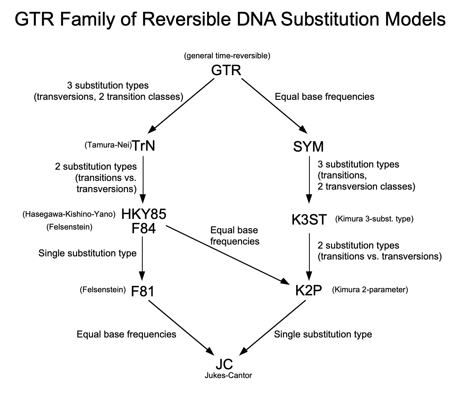
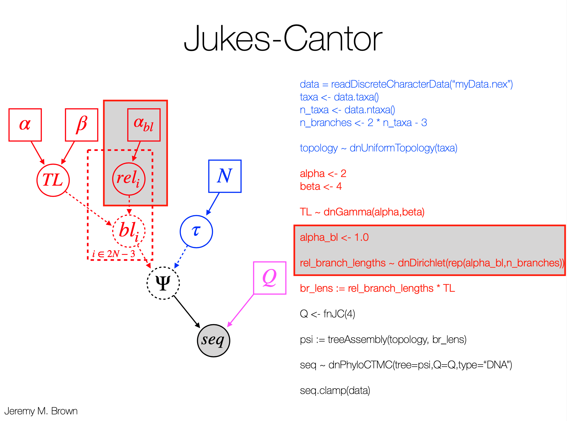

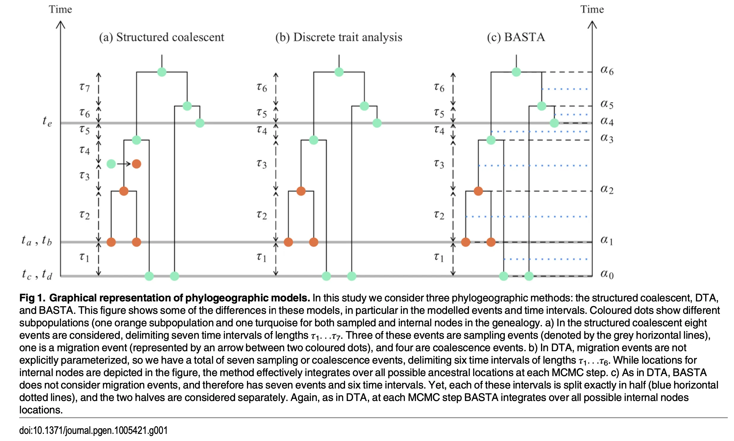
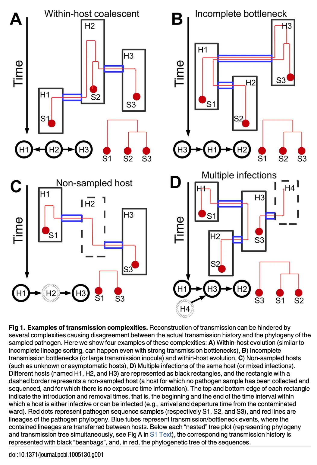
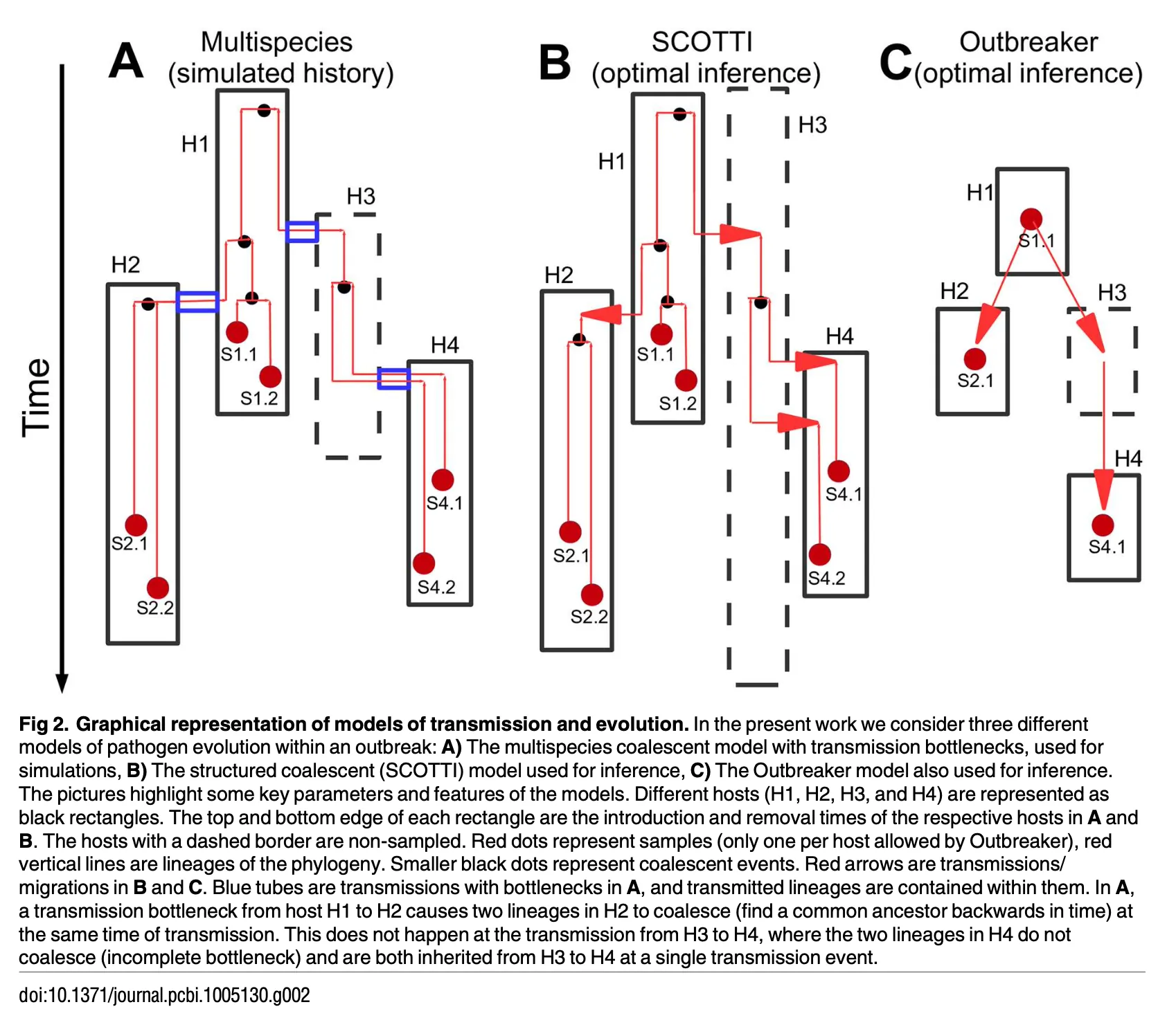
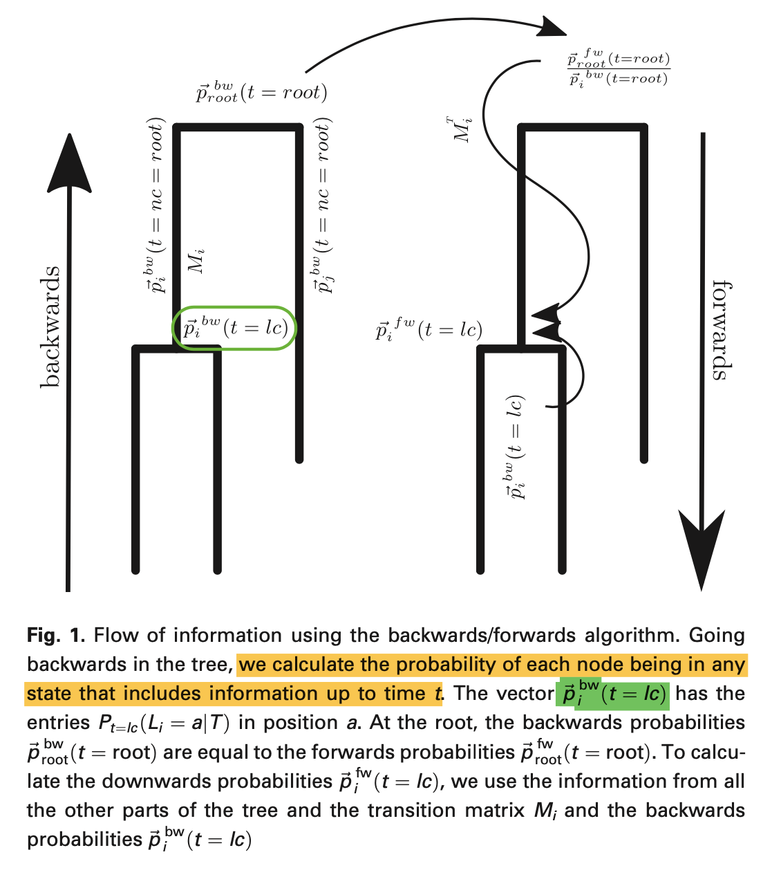
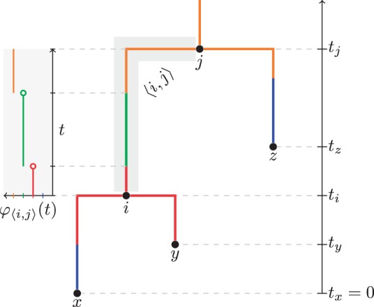
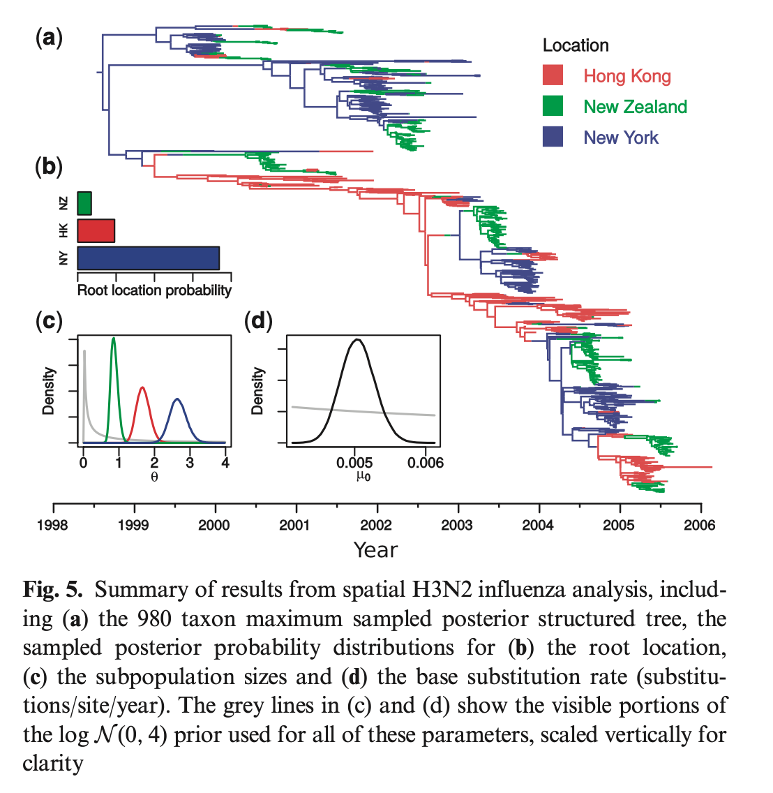


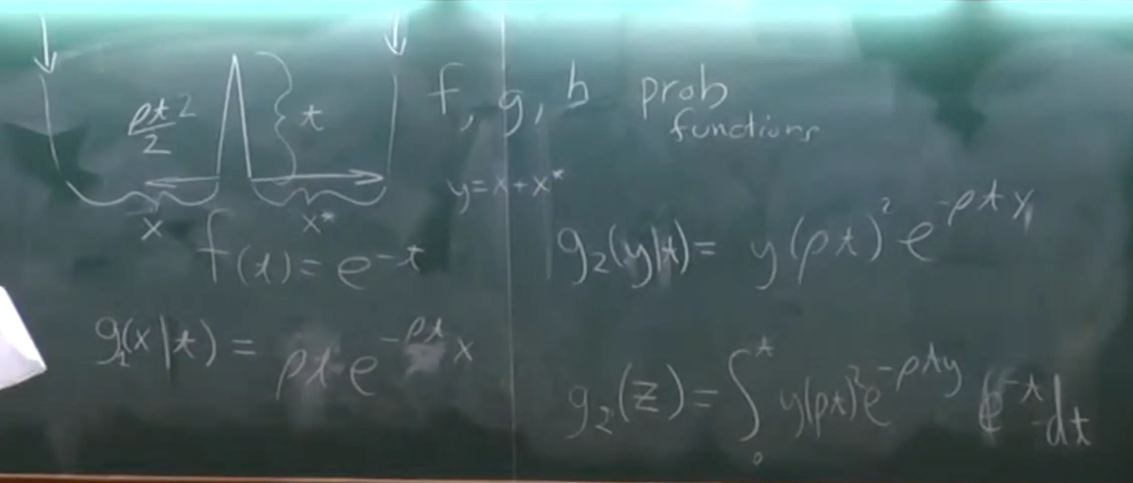
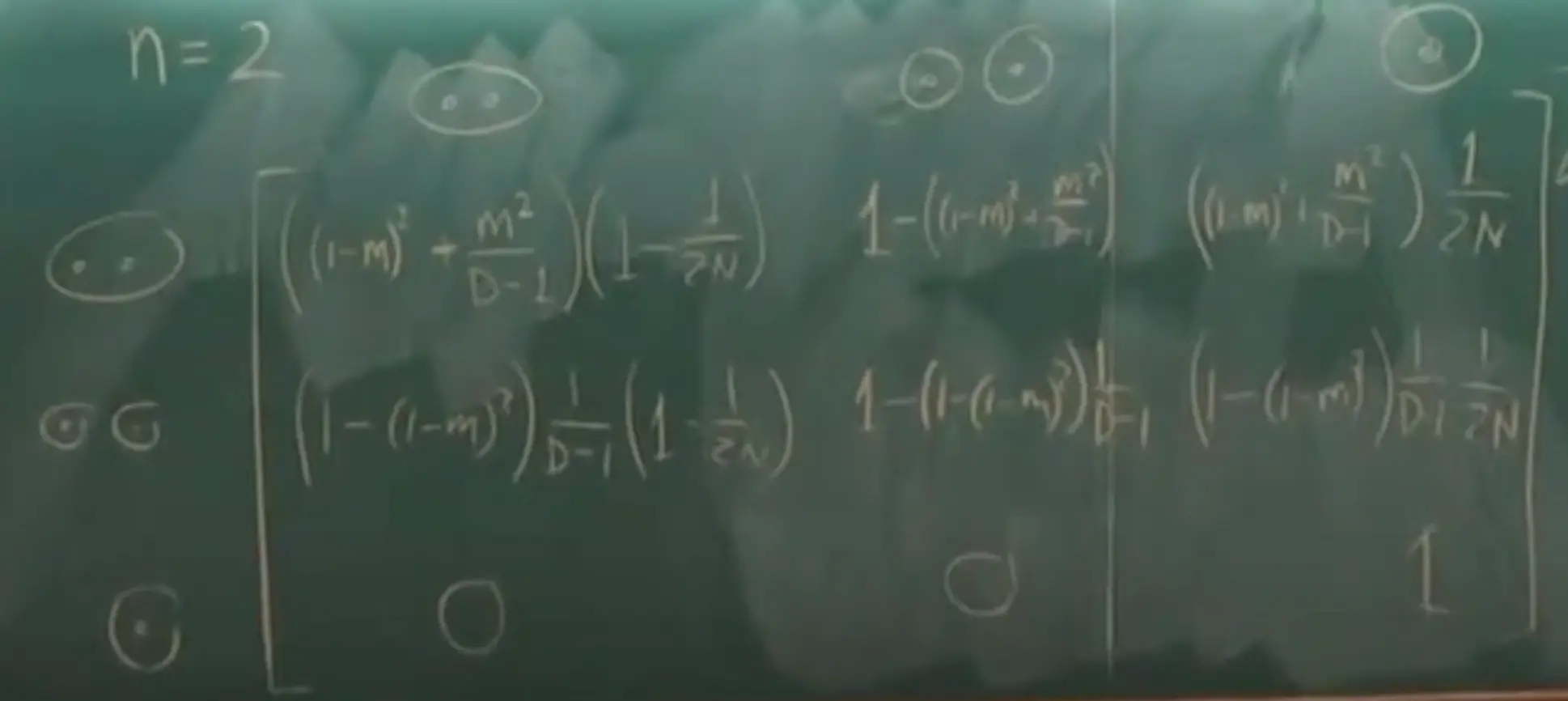
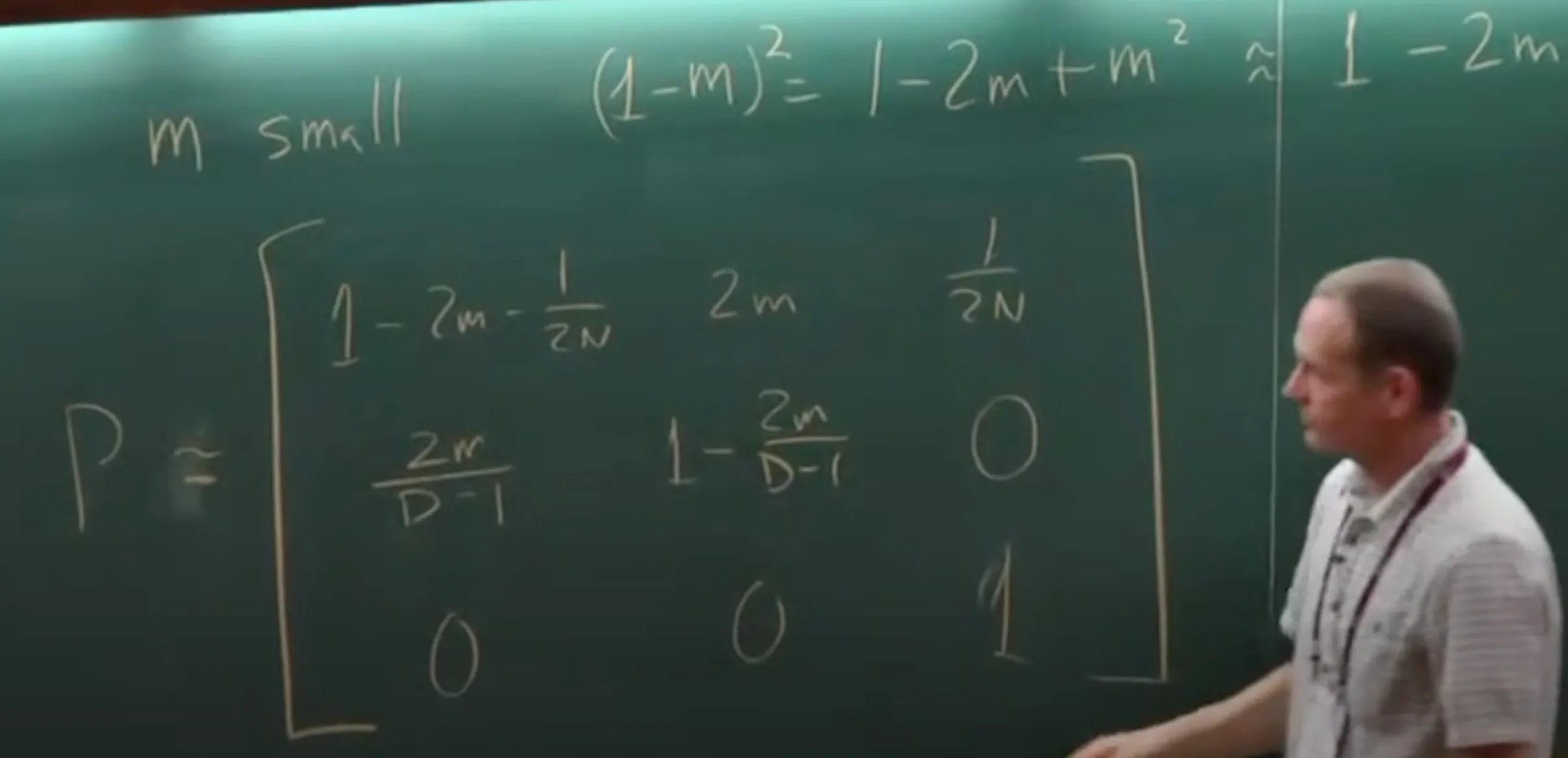
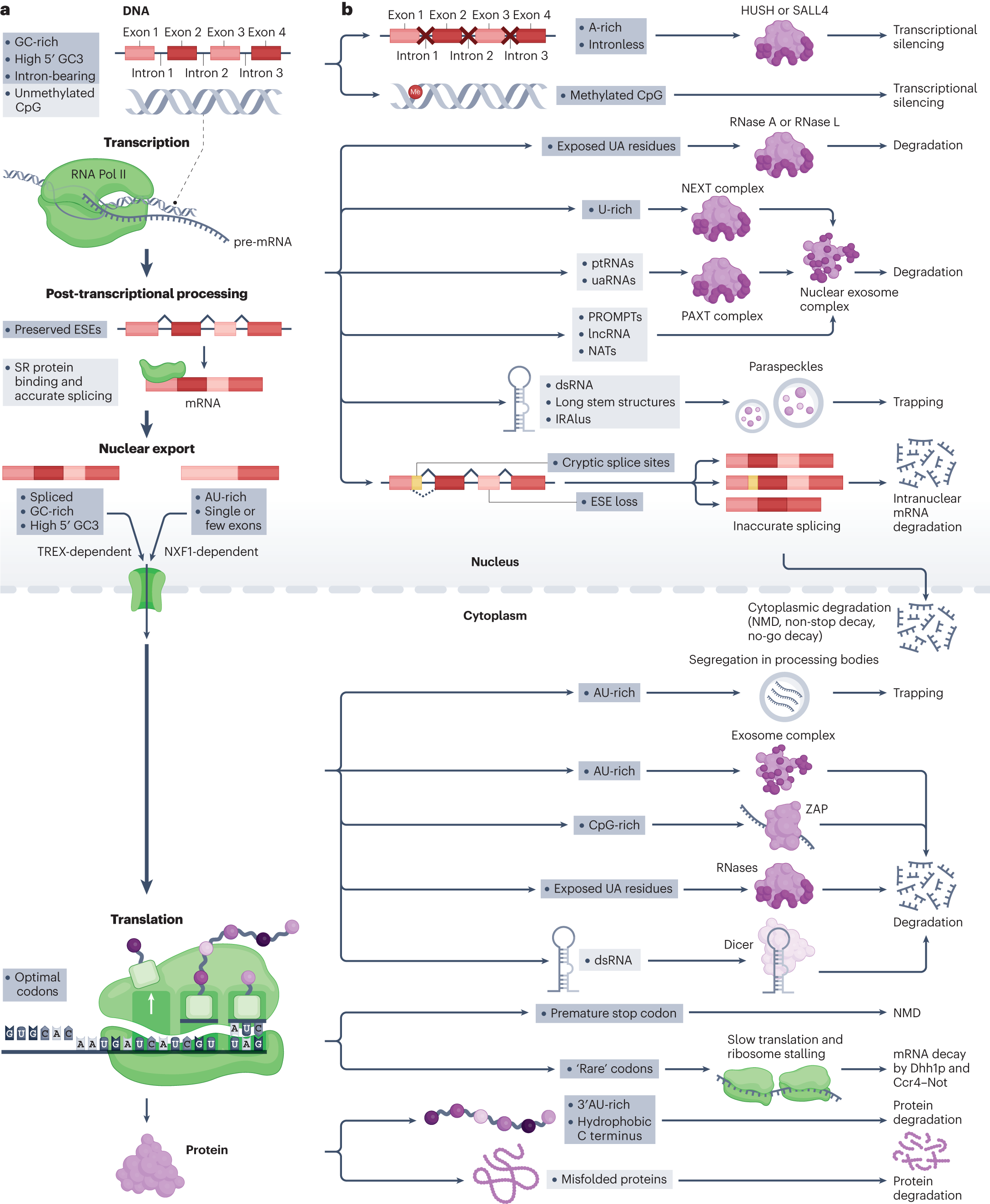
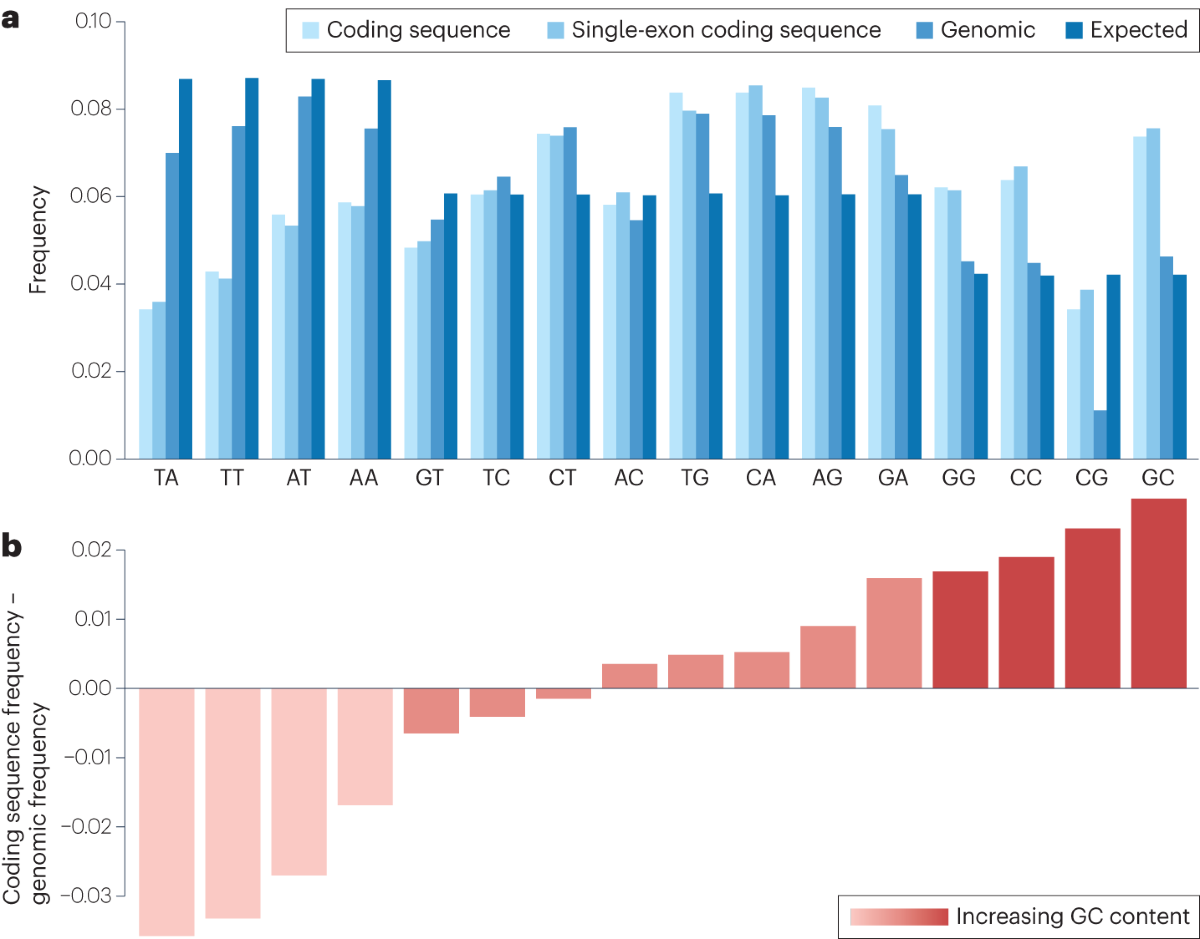