
Book notes: Introduction to Probability (Dimitri P. Bertsekas and John N. Tsitsiklis, 2008)
Last modified:This post records the notes when I read Introduction to Probability by Dimitri P. Bertsekas and John N. Tsitsiklis.
Sample Space and Probability
Probabilistic models
- Sample space must be collectively exhaustive, i.e., different elements of the sample space should be distinct and mutually exclusive. The sample space is usually denoted Ω.
Conditional probability
- The Monty Hall Problem, Switch to the other unopened door will result in 2/3 probability of winning.
Total probability theorem and Bayes’ rule
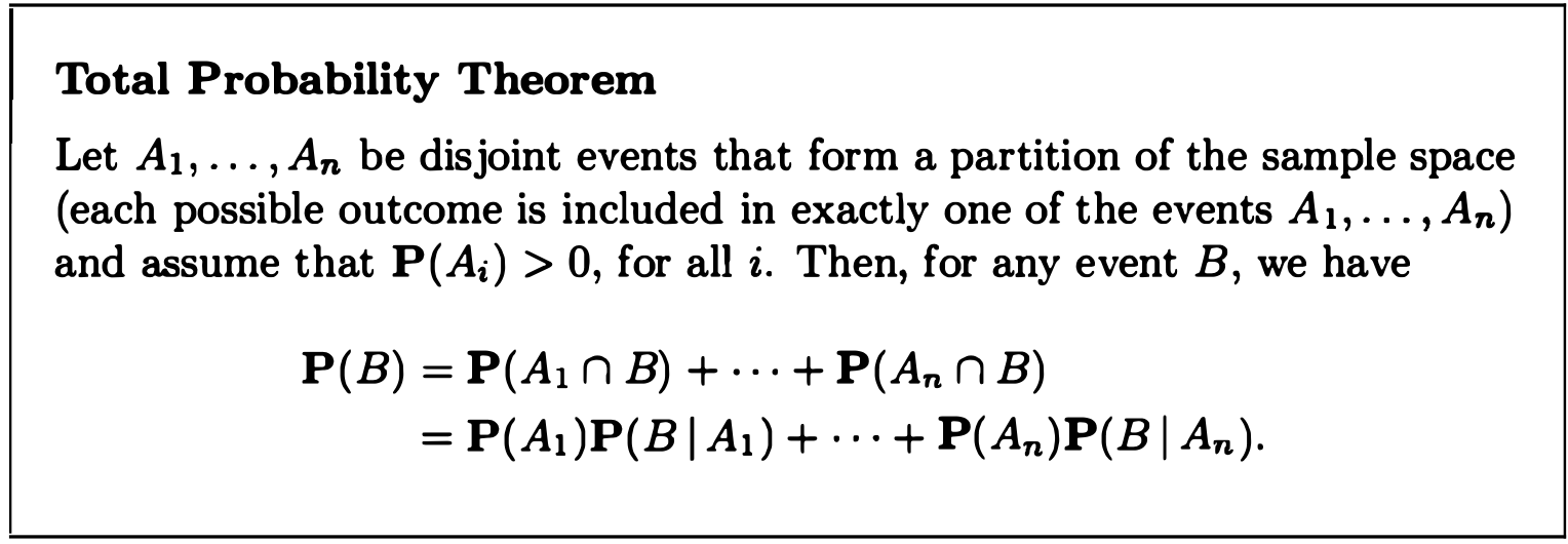
- Total Probability Theorem
-
Bayes’ Rule
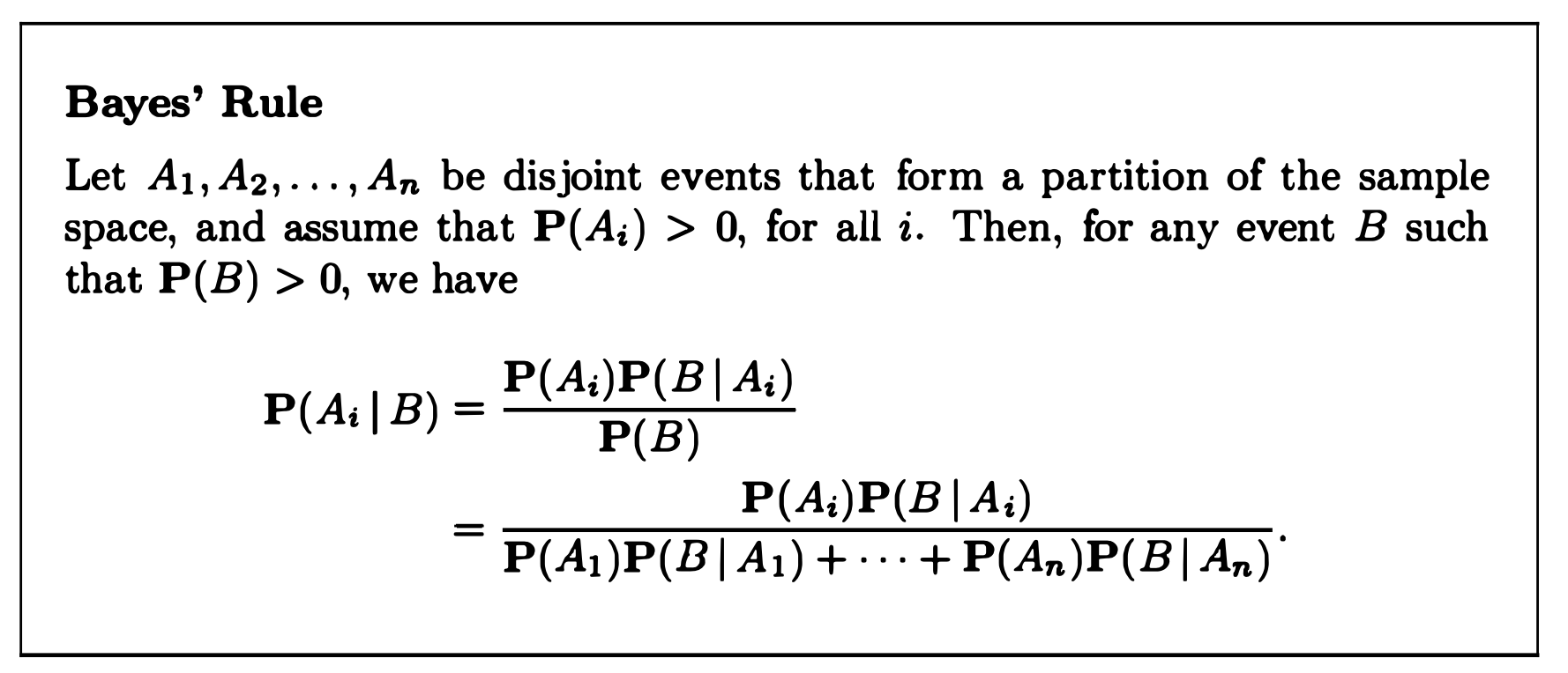
Posterior and prior probability: Given that the effect $B$ has been observed, we wish to evaluate the probability $P(A_i B)$ that the cause $A_i$ is present. We refer to $P(A_i B)$ as the posterior probability of event $A_i$ given the information, to be distinguished from $P(A_i)$, which we call the prior probability.
Independence and counting
-
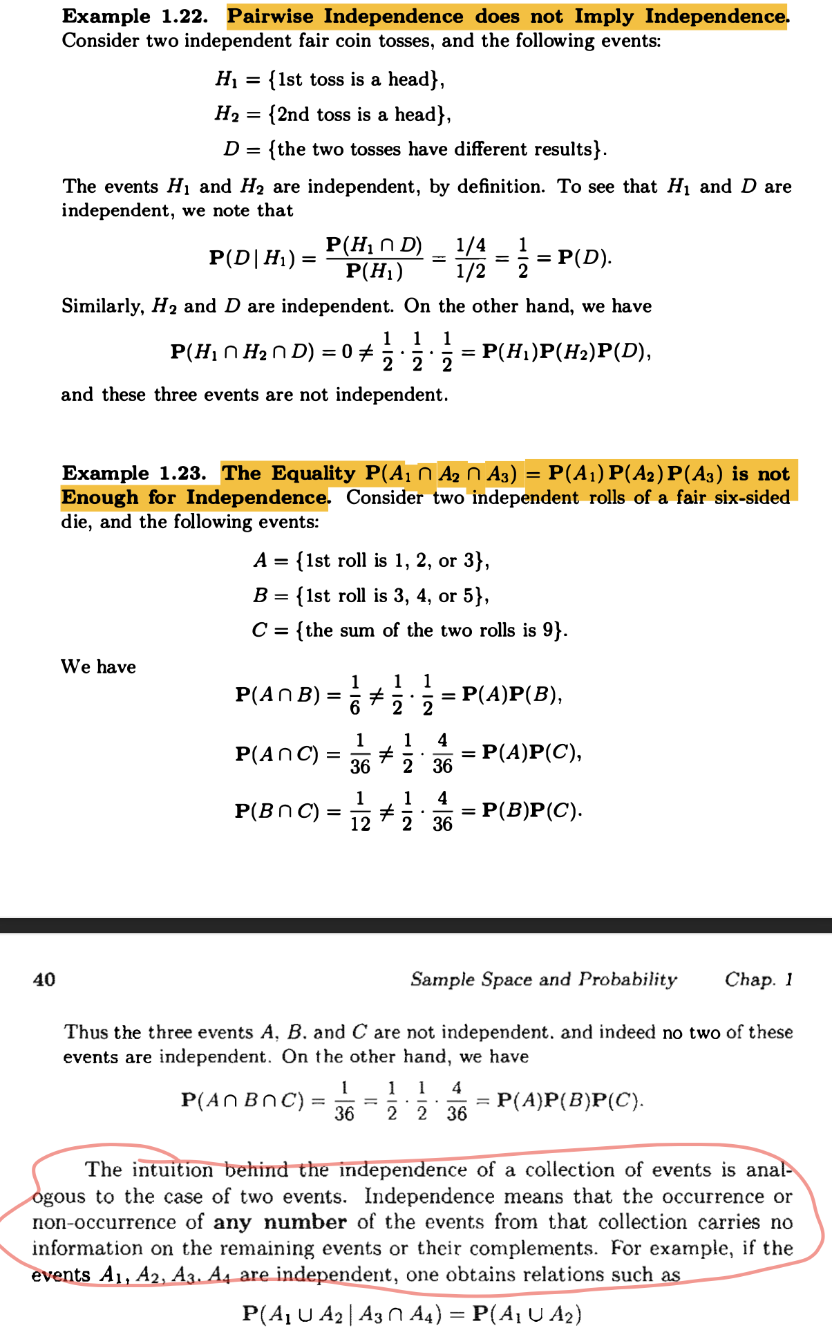
A very important point here is that we usually test the independence numerically, rather than logically, see below:
-
Independent Bernoulli trials form Binomial model. Note that the binomial probabilities add to 1, thus showing the binomial formula: $\sum_{k=0}^n{n \choose k}p^k(1-p)^{n-k}=1$. In the special case where $p=0.5$, this formula becomes $\sum_{k=0}^n{n \choose k}=2^n$. This equal to the number of all subsets of an n-element set. which is $2^n$ (全子集问题:针对每一个元素,都有取或不取两个选择,因此总共的不同的子集数量为$2^n$).
-
If the order of selection matters, the selection is called a permutation, and otherwise, it is called a combination.
-
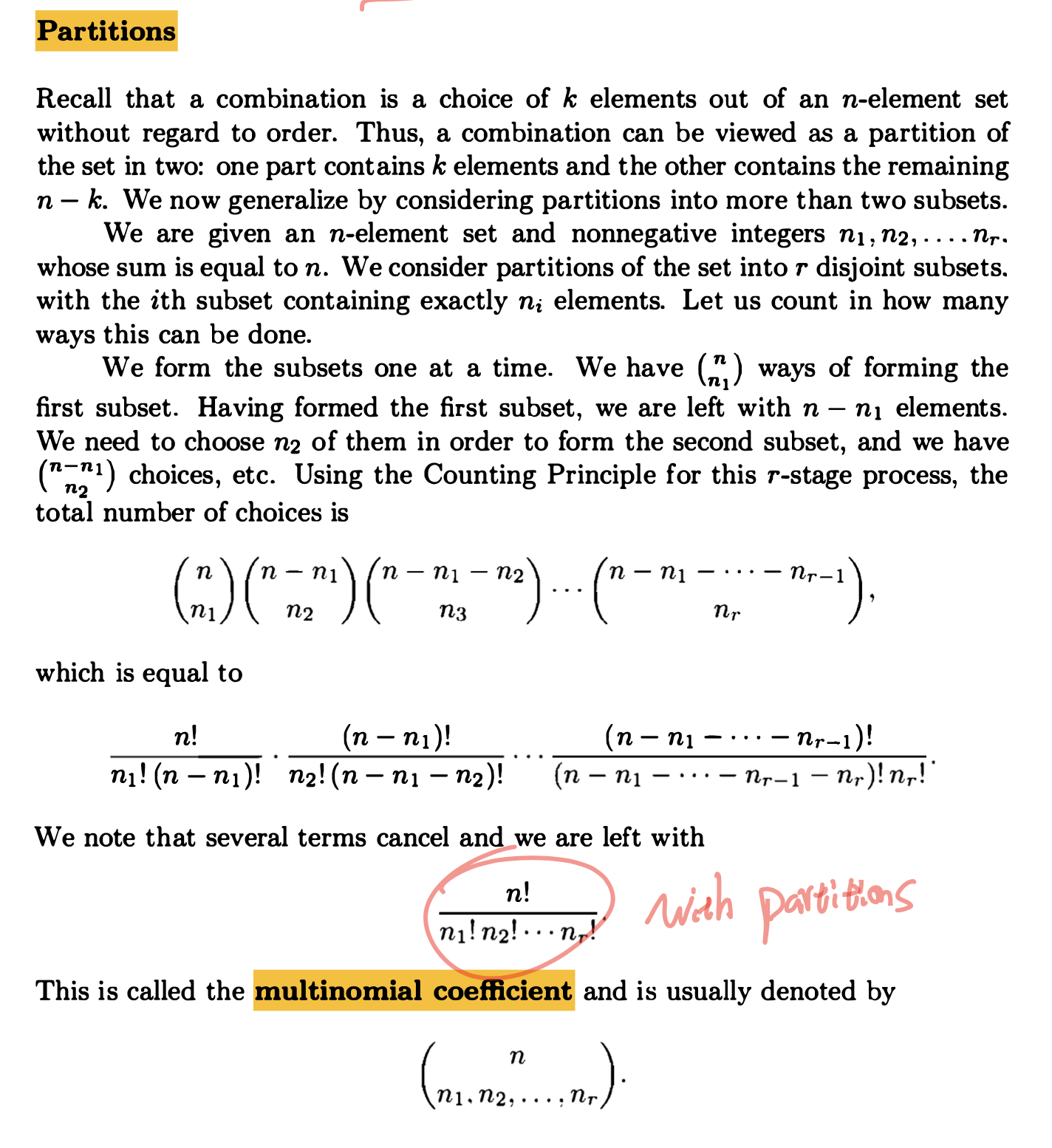
Partitions:
-
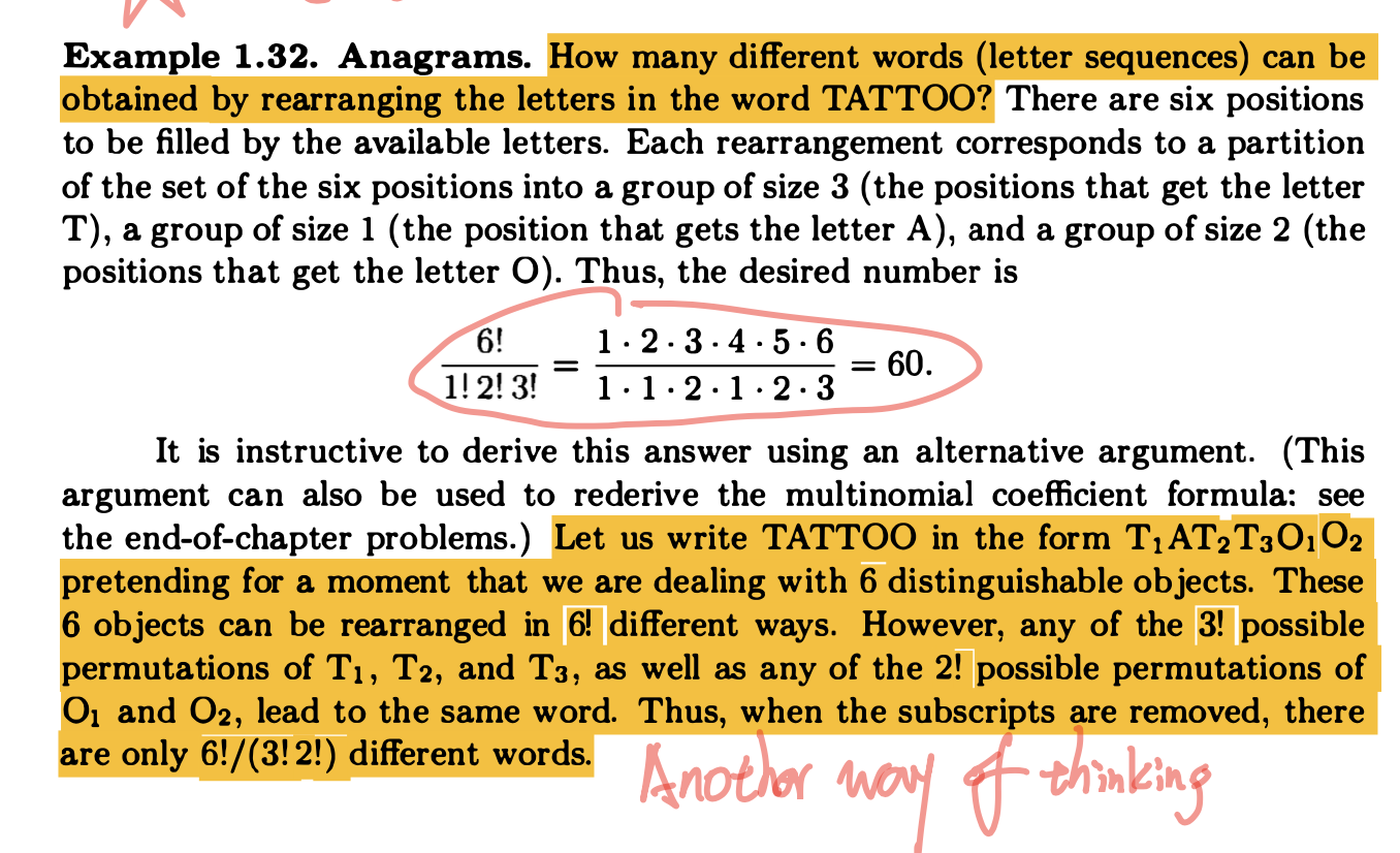
A very useful example: How many different words (letter sequences) can be obtained by rearranging the letters in the word TATTOO?
-
The above question have a similar application in genomic study, how many different synonymous genomes can be obtained by swapping the synonymous codons in the genome?
Discrete random variables
Basic concepts
- Mathematically, a random variable is a real-valued function of the experimental outcome (Random variables must have explicit numerical values). Thus, a function of a random variable defines another random variable (e.g. one can constrcut Binomial random variable with Bernoulli random variable).
- A random variable is called discrete if its range (the set of values taht it can take) is either finite or countably infinite.
- A discrete random variable has an associated probability mass function (PMF). which gives the probability of each numerical value that the random variable can take.
Probability mass functions
-
Discrete uniform over $[a,b]$: \(p_X(k)= \begin{cases} & \frac{1}{b-a+1}, & \text{if } k = {a, a+1, ..., b},\\ & 0, & Otherwise,\\ \end{cases}\).
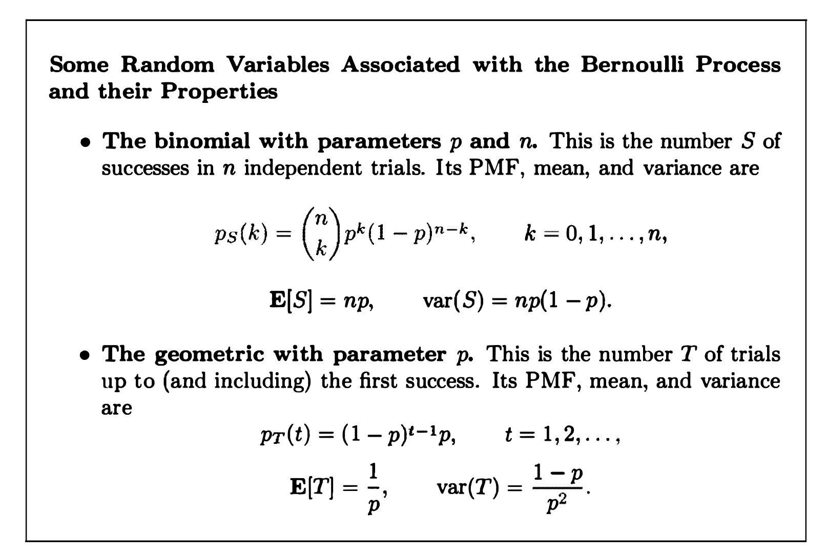
- The binomial random variable is the number of heads X in the n-toss sequence : $P(X=k)={n \choose k}p_k(1-p)^{n-k},k=0,1,…,n.$
- The geometric random variable is the number X of tosses needed for a head to come up for the first time: $P(X=k)=(1-p)^{k-1}p, k=1,2,…$. Also note that the sum of geometric sequence $S_n=\sum_{k=0}^{\infty}p^k=\frac{1-p^{n+1}}{1-p}$ (using $pS_n - S_n$ to derive this), so when $n \to \infty$ it becomes $\frac{1}{1-p}$. Thus, sum of the PMF: $\sum_{k=1}^{\infty}(1-p)^{k-1}p=p\sum_{k=0}^{\infty}(1-p)^k=p\frac{1}{1-(1-p)}=1.$
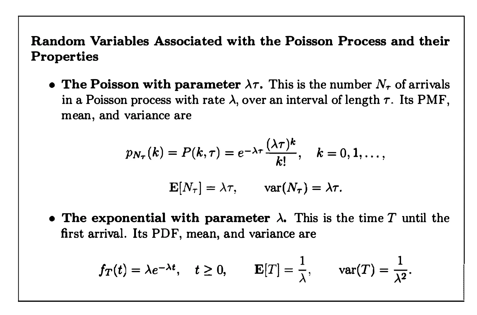
- The Poisson random variable is the number X of success (small $p$) in (large $n$) total events. The PMF: $P(X=k)=e^{-\lambda}\frac{\lambda^k}{k!}, k=0,1,2,…$ where $\lambda$ is a positive parameter, I tend to think $\lambda$ as the expected number of success for each individual ($np$). The Poisson PMF can approximate the binomial PMF when $n$ is large and $p$ is small. Using Poisson PMF may result in simpler model and calculation.
Expectance and variance
Expectance: $E[g(X)] = \sum_xg(x)p_X(x)$ Variance: $var(X) = \sum_x(E[X]-x)^2p_X(x)$ A convenient alternative formula: $var(X) = -(E[X])^2 + E[X^2]$
Mean and variance of some common random variables
-
Discrete uniform over $[a,b]$: \(E(X)=\frac{a+b}{2},\\ var(X)=\frac{(b-a)(b-a+2)}{12}.\)
-
Bernoulli: \(E[X] = p,\\ E[X^2] = 1^2 \times p+0^2 \times (1-p)=p,\\ var(X) = (1-p)^2p+p^2(1-p)=p(1-p)(1-p+p)=p(1-p).\)
-
Binomial: Since Binomial random variable is the sum of $n$ independent Bernoulli random variables, the $E(X) = np$ and $var(X) = np(1-p)$.
-
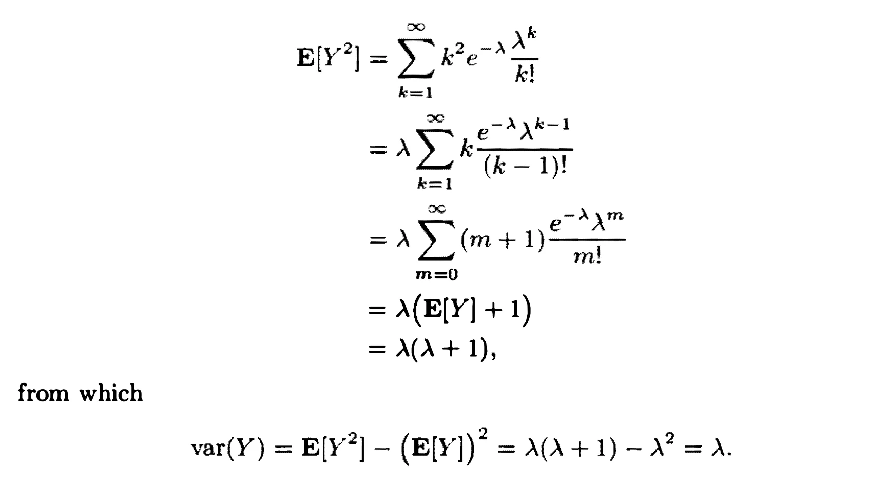
Poisson: Since a Poisson random variable can be viewed as the “limit” of the binomial random variable as $n \to \infty$ and $p \to 0$, we can informally obtain the mean and variance of the Poisson via Binomial: $E(X)=var(X)=\lambda$. We can also verify this by:
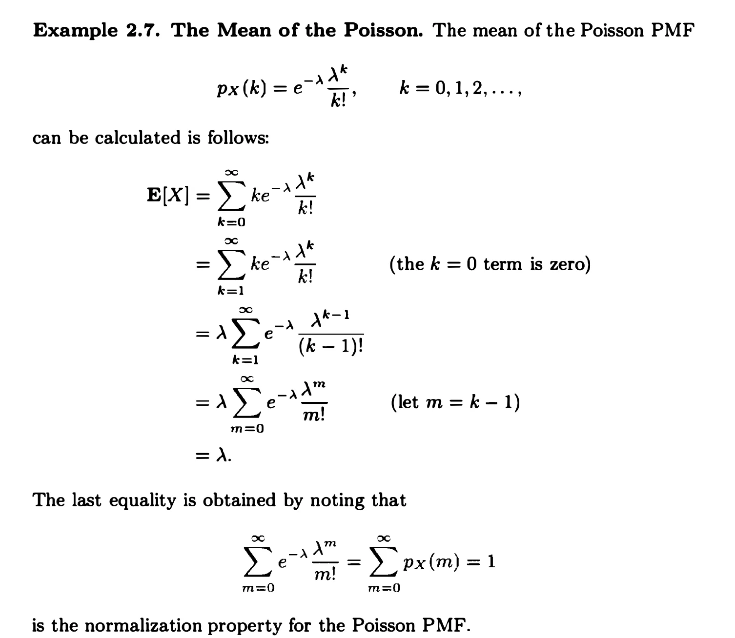
and
-
Geometric: \(E[X]=\sum_{k=1}^{\infty}k(1-p)^{k-1}p\\ var(X)=\sum_{k=1}^{\infty}(k-E[X])^2(1-p)^{k-1}p\) This can be calculated by applying the the total expectation theorem: \(\begin{align} E[X]&=P(X=1)E[X|X=1]+P(X>1)E[X|X>1]\\ &=p+(1-p)(1+E[X])\\ \end{align}\\ \Rightarrow E[X]=\frac{1}{p}\) and \(\begin{align} E[X^2]&=P(X=1)E[X^2|X=1]+P(X>1)E[X^2|X>1]\\ &=p+(1-p)(E[(1+X)^2])\\ &=p+(1-p)(1+2E[X]+E[X^2])\\ \end{align}\\ \Rightarrow E[X^2]=\frac{2}{p^2}-\frac{1}{p}\\ \Rightarrow var(X)=E[X^2]-(E[X])^2=\frac{1-p}{p^2}\)
-
Sample mean: Consider a random variable $S_n$ which represents sample mean of independent random variables $X_i$ (e.g. Bernoulli). \(S_n = \frac{X_1 + X_2+...+X_n}{n}\\ E(S_n)=p\\ var(S_n)=\frac{n\times var(X)}{n^2}=\frac{p(1-p)}{n}\)
Joint PMFs and conditional PMFs
The marginal PMFs can be obtained from the joint PMF, using the formulas: $p_X(x)=\sum_yp_{X,Y}(x,y)$, $p_Y(y)=\sum_xp_{X,Y}(x,y)$.
The conditional PMF of X given Y can be calculated through: $p_X(x)=\sum_yp_{Y}(y)p_{X|Y}(x|y)$.
General random variables
Continuous Random Variables, PDFs and CDFs
- Continuous Uniform random variable: \(f_X(x)= \begin{cases} \frac{1}{b-a}, & \text{if } a\le x \le b, \\ 0, & Otherwise, \\ \end{cases}, \\ E[X] = \int_{-\infty}^{\infty}xf_X(x)dx=\int_a^bx\cdot\frac{1}{b-a}dx=\frac{a+b}{2},\\ E[X^2] = \int_a^b \frac{x^2}{b-a}dx=\frac{a^2+ab+b^2}{3},\\ var(X) = E[X^2]-(E[X])^2 = \frac{(b-a)^2}{12}.\)
- Exponential random variable (the amount of time until an incident of interest takes place):
\(f_X(x)= \begin{cases}
\lambda e^{-\lambda x}, & \text{if } x\ge0, \\
0, & Otherwise, \\
\end{cases}, \\
P(x\ge 0)=\int_0^{\infty}\lambda e^{-\lambda x}dx = -e^{-\lambda x}\bigg|_0^{\infty}=1, \\
P(x\ge a)=e^{-\lambda a}, \\
E[X] = \frac{1}{\lambda},\\
var(X)=\frac{1}{\lambda^2}.\)
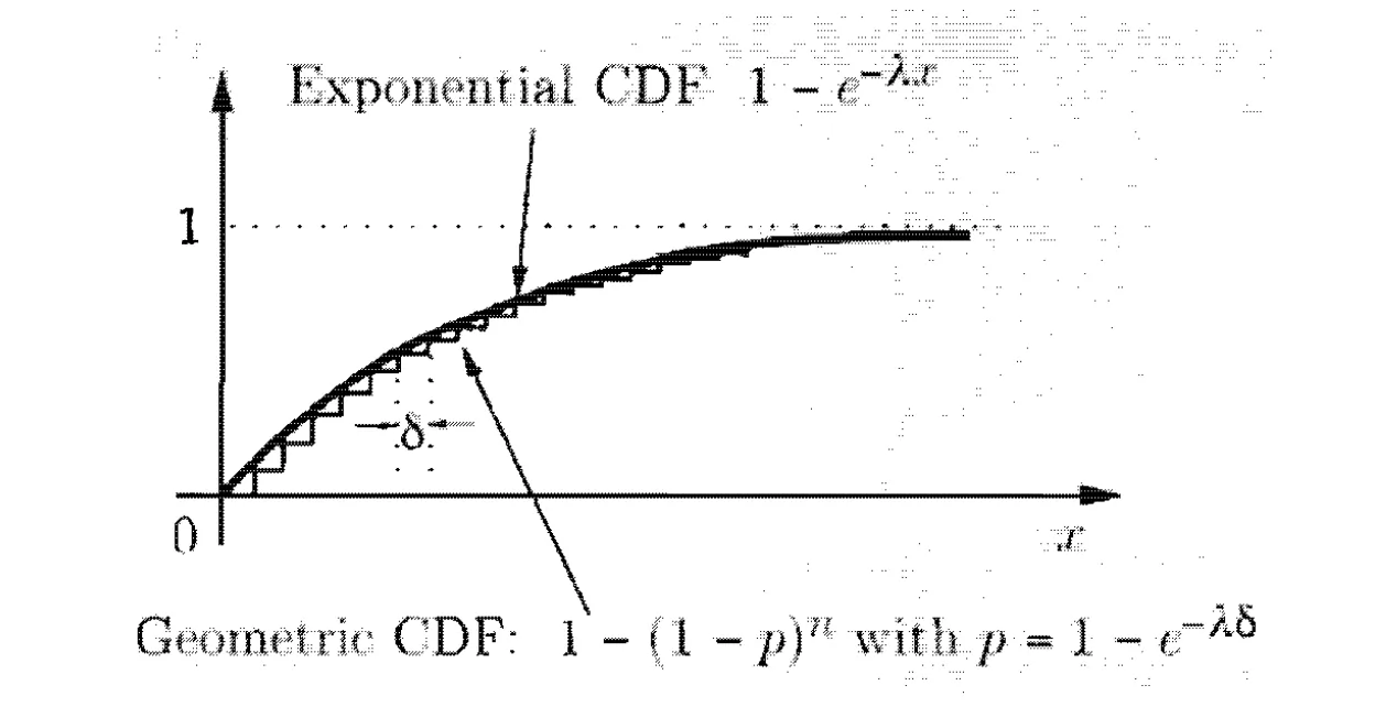
The CDF between geometric and exponential random variables are similar:
Normal (Gaussian) random variables
A continuous random variable $X$ is said to be normal or Gaussian if it had the following PDF: \(f_X(x)=\frac{1}{\sqrt{2\pi}\sigma}e^{-(x-\mu)^2/2\sigma^2},\\ E[X]=1,\\ var(X)=\sigma^2.\)
The normality is preserved by linear transformation: \(Y=aX+b\\ E[Y]=aE[X]+b\\ var(Y)=a^2var(X)\) A standard normal random variable is a normal random variable with zero mean and unit variance, with the CDF: \(\Phi(y) = P(Y\le y)=\frac{1}{\sqrt{2\pi}}\int_{-\infty}^{y}e^{-t^2/2}dt\) A normal random variable $X$ with mean $\mu$ and variance $\sigma^2$ can be “standardized” by linear transformation: \(Y=\frac{X-\mu}{\sigma}\\ E[Y]=\frac{E[X]-\mu}{\sigma}=0,\\ var(Y)=\frac{var(X)}{\sigma^2}=1,\\\) Normal random variables play an important role in a broad range of probabilistic models, becasue the sum of a large number of independent and identically distributed (not necessarily normal) ran dom variables has an approximately normal CDF (the central limit theorem).
joint PDFs and conditional PDFs
Buffon’s Needle is a famous example of joint uniform PDFs.
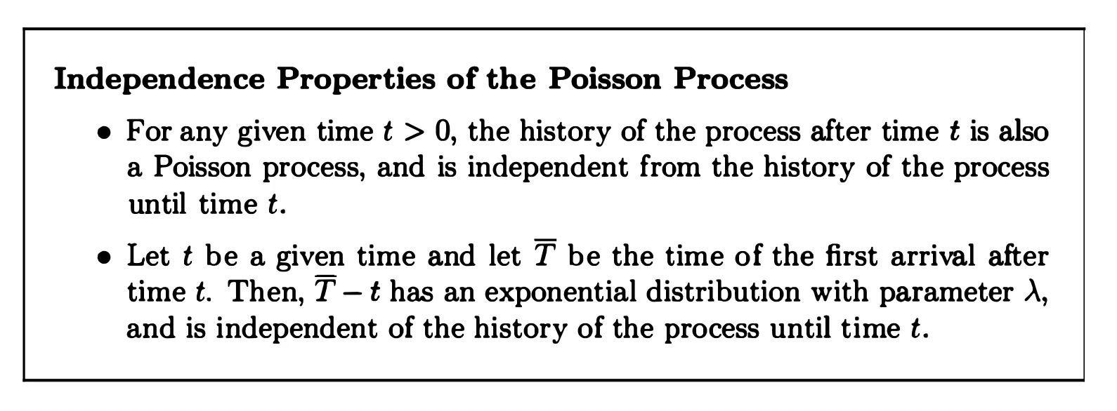
The Exponential Random Variable is Memoryless, 例如你抛了十次硬币都是反面, 前面十次的结果不影响你下一次正面出现的等待时间.
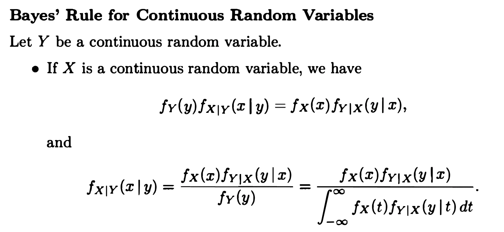
The continuous Bayes’s Rule
Further topics on random variables
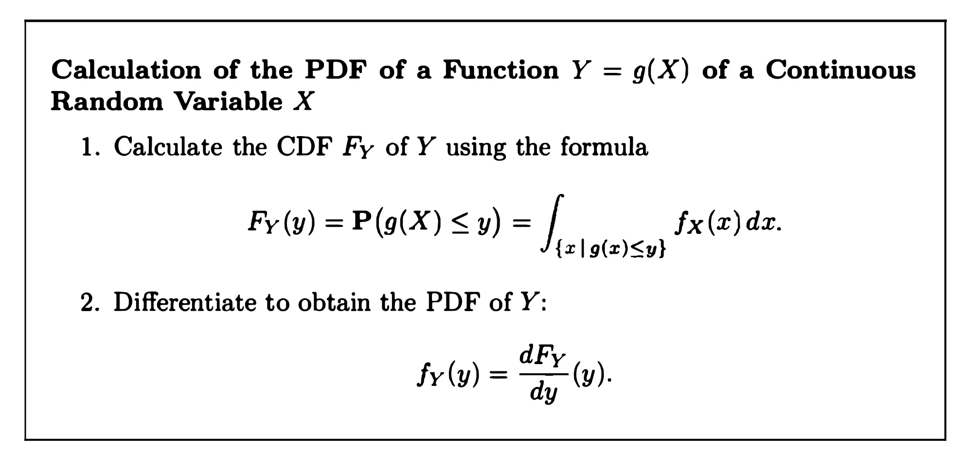
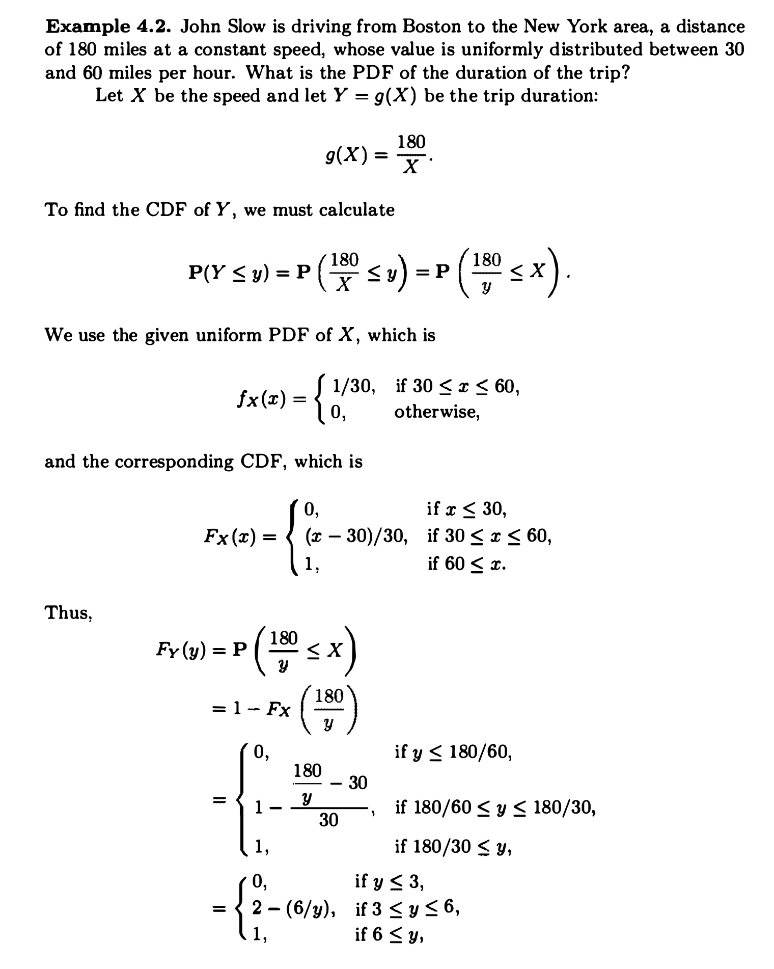
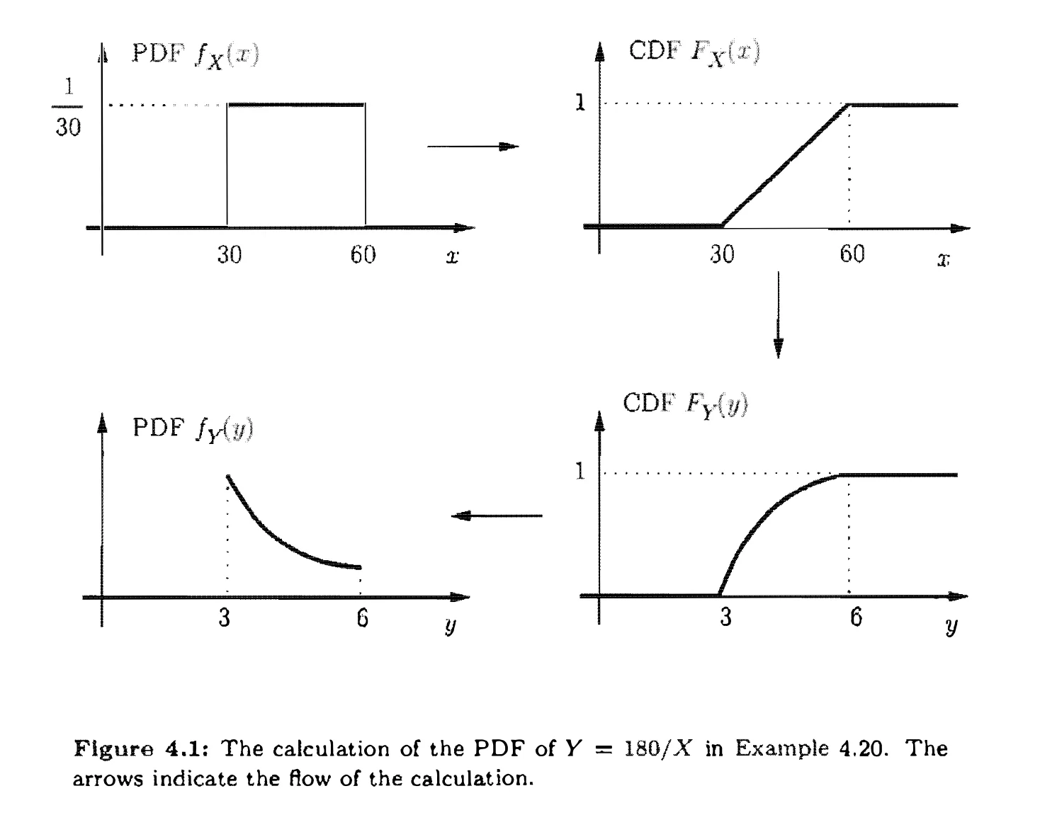
Derived distributions
The principal method for calculating a derived distribution is the following two-step approach.
For two Random Variables, such as for two exponential random variables $X$ and $Y$, and we want to find the PDF of $Z = X-Y$. This is known as a two-sided exponential PDF, also called the Laplace PDF.
Sums of Independent Random Variables - Convolution: $Z=X+Y$.
The sum of two independent uniform random variables has a triangular shape.
The sum of two independent normal random variables is normal (with mean $\mu_x+\mu_y$ and variance $\sigma_x^2+\sigma_y^2$).
Covariance and correlation
\(Cov(X, Y)=E[(X-E[X])(Y-E[Y])]\\ Cov(X,Y)=E[XY]-E[X]E[Y]\\\) The sign of the correlation coefficient $\rho(X, Y)=\frac{Cov(X,Y)}{\sqrt{var(X)var(Y)}}$ is determined by $Cov(X,Y)$, suggesting a positive or negative correlation, the size of $|\rho|$ provides a normalized measure of the extent to which this is true.
$var(X_1 + X_2) = var(X_1) + var(X_2) + 2cov(X_1, X_2)$
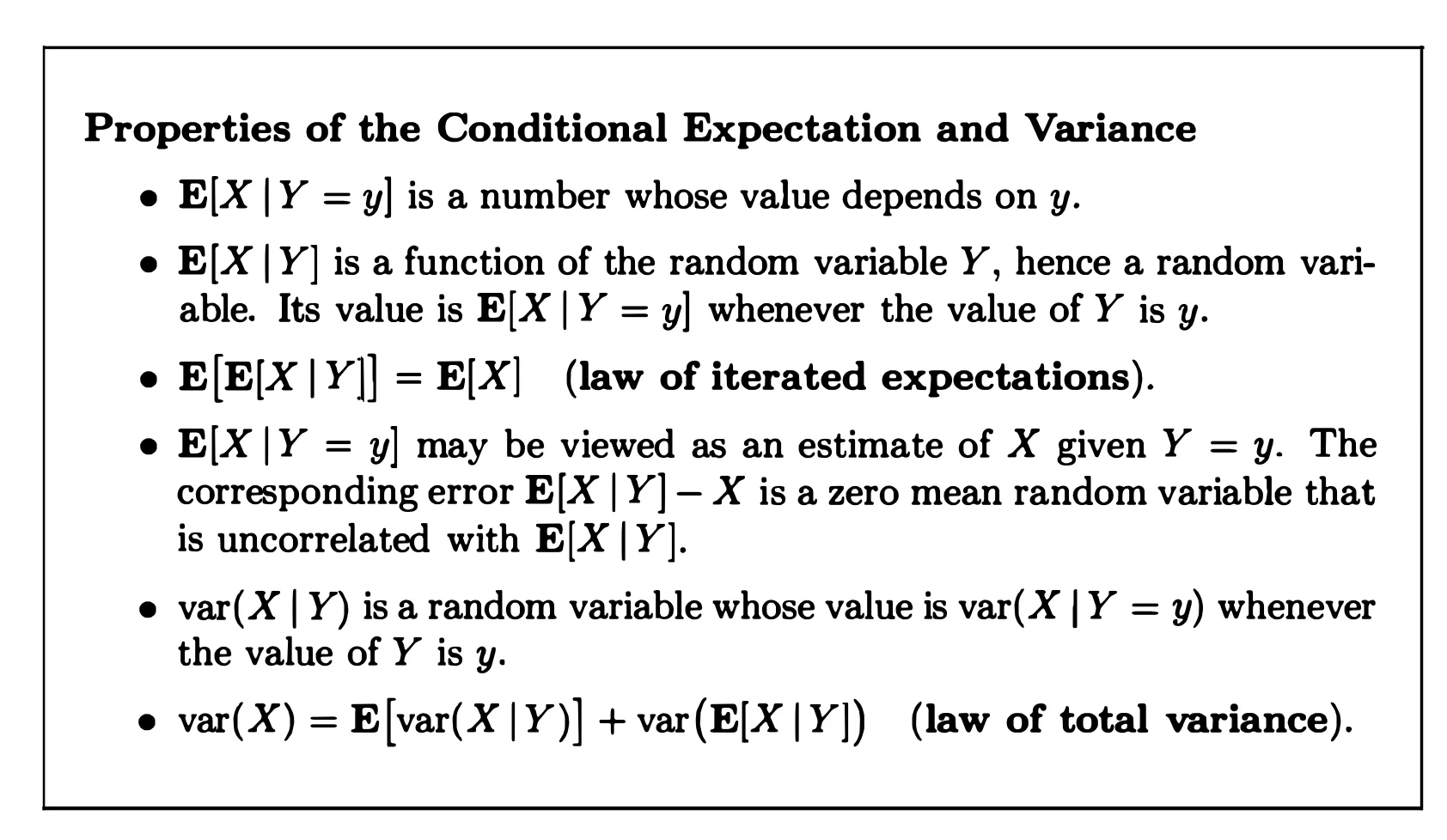
Conditional expectation and variance revisited
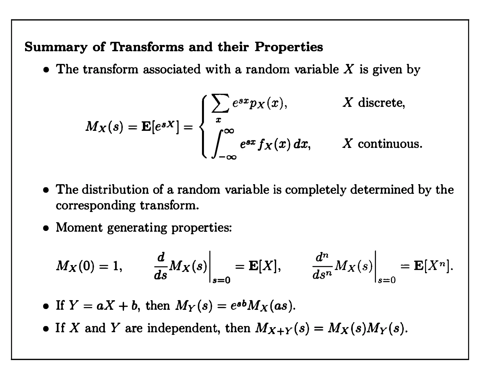
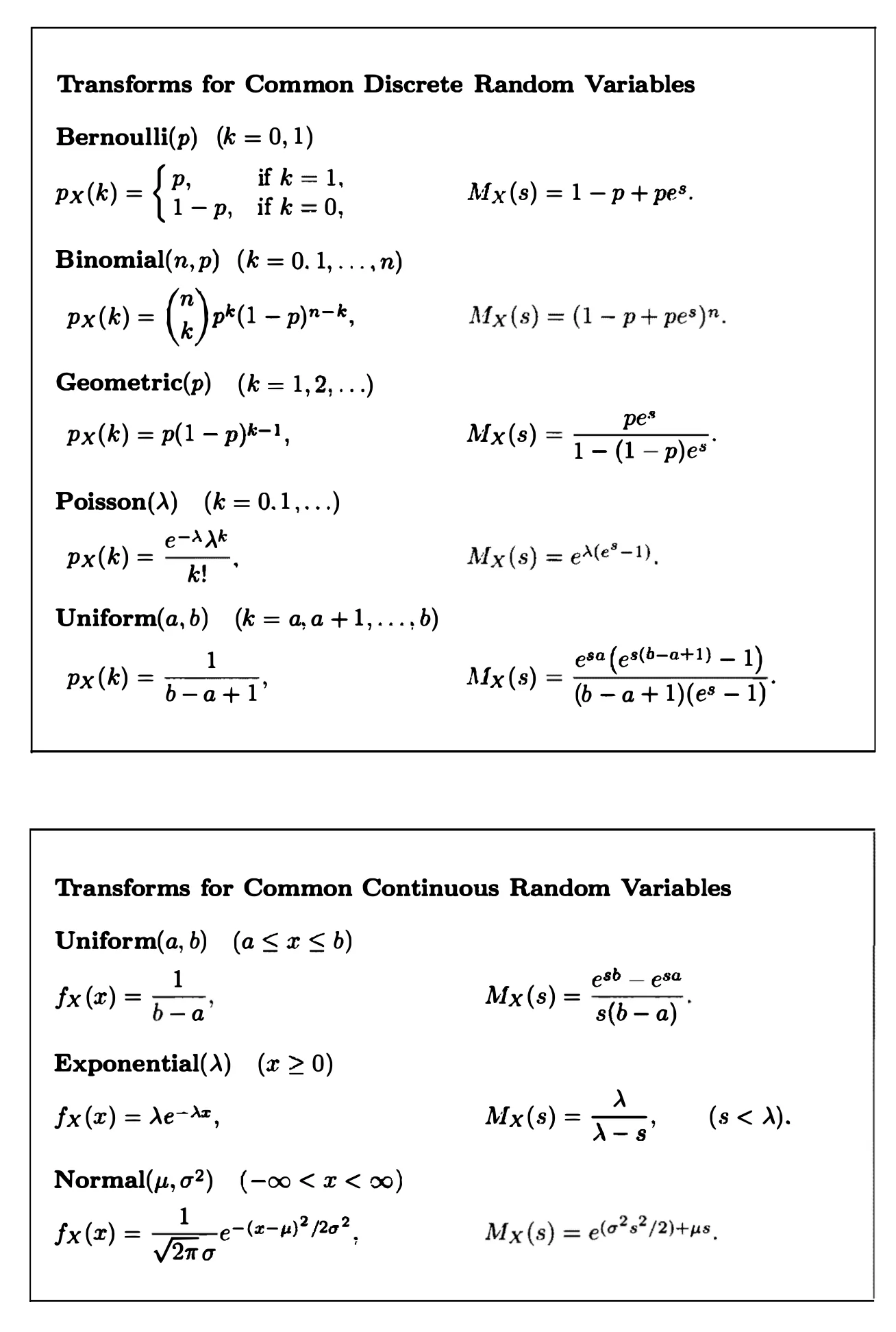
Transforms
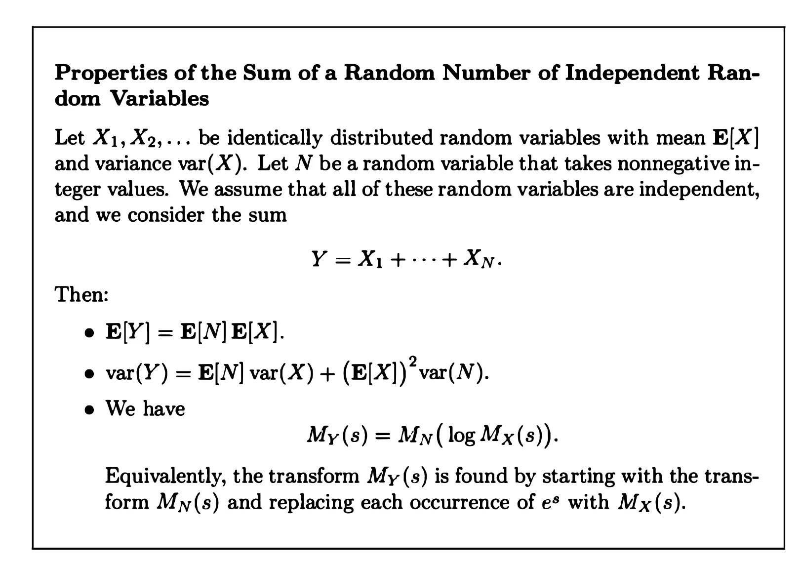
Sum of random number of independent random variables
Limit Theorems
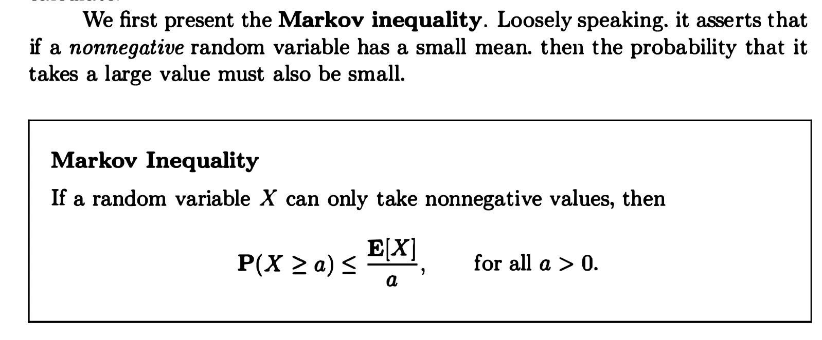
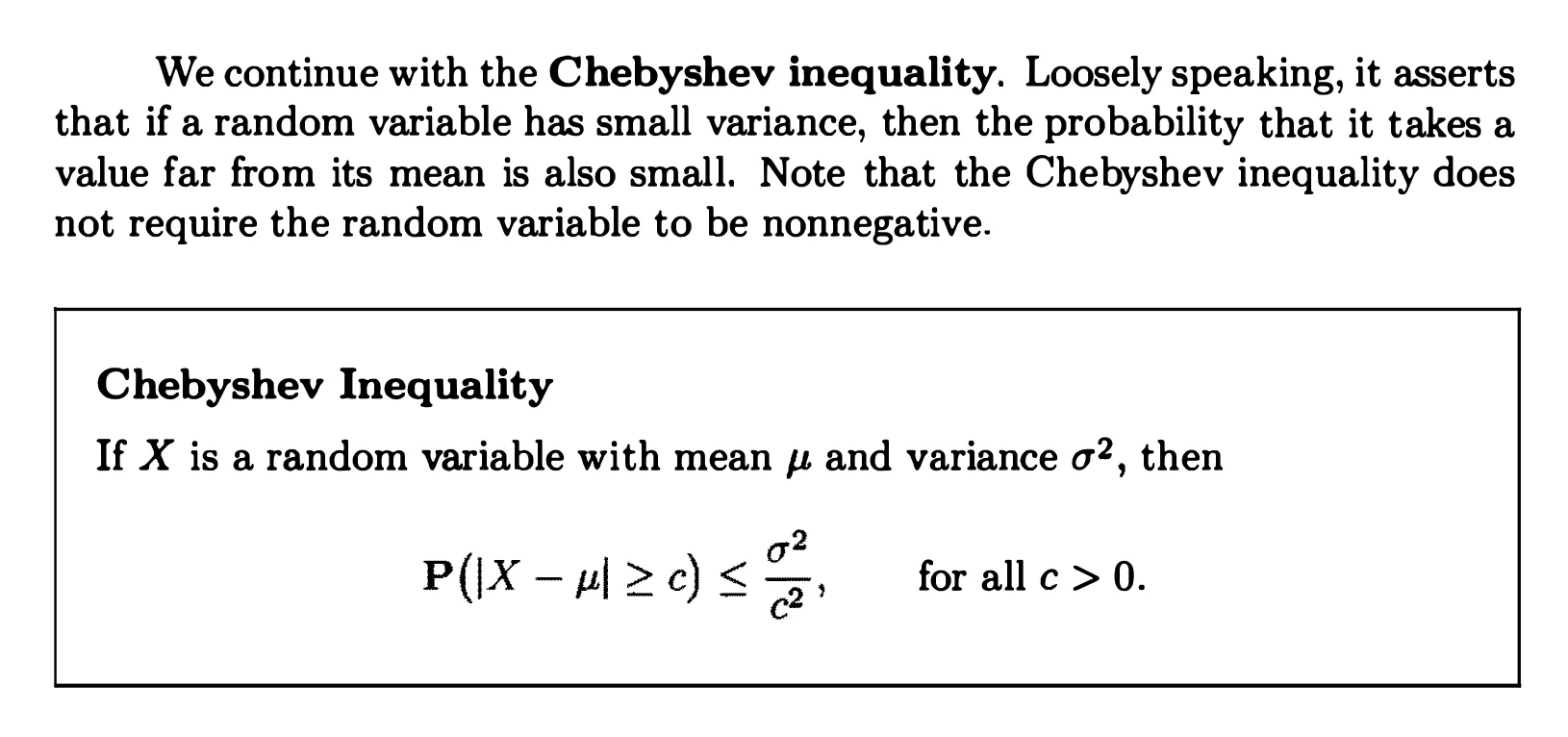
Markov and Chebyshev Inequalities
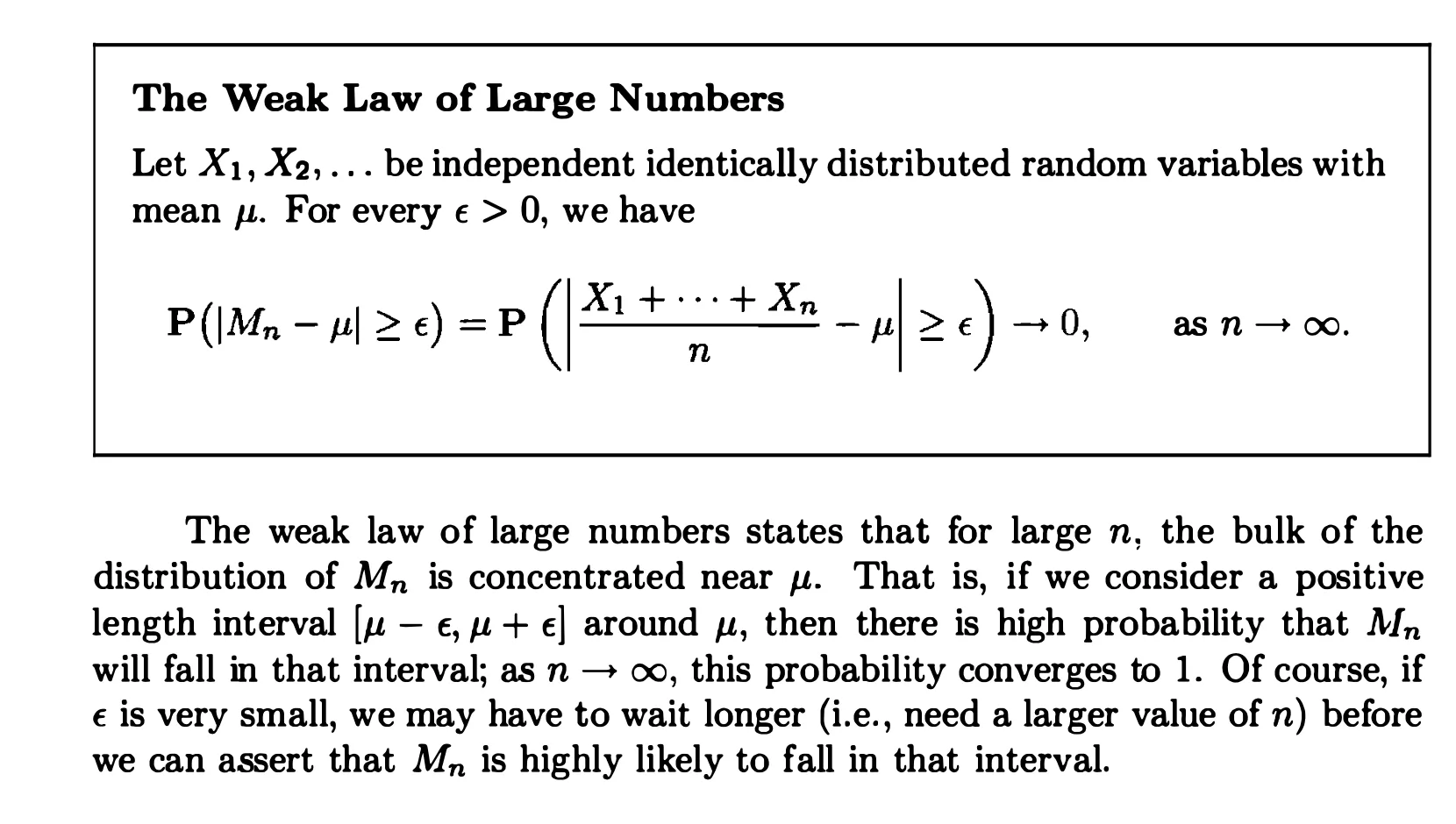
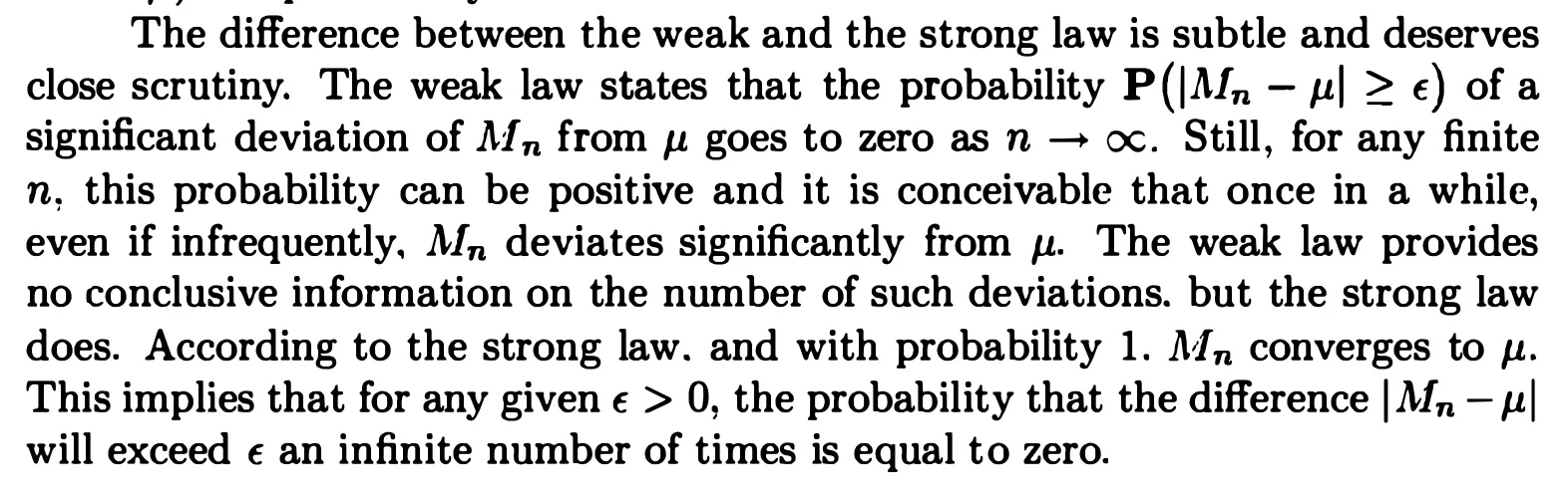
THE WEAK LAW OF LARGE NUMBERS
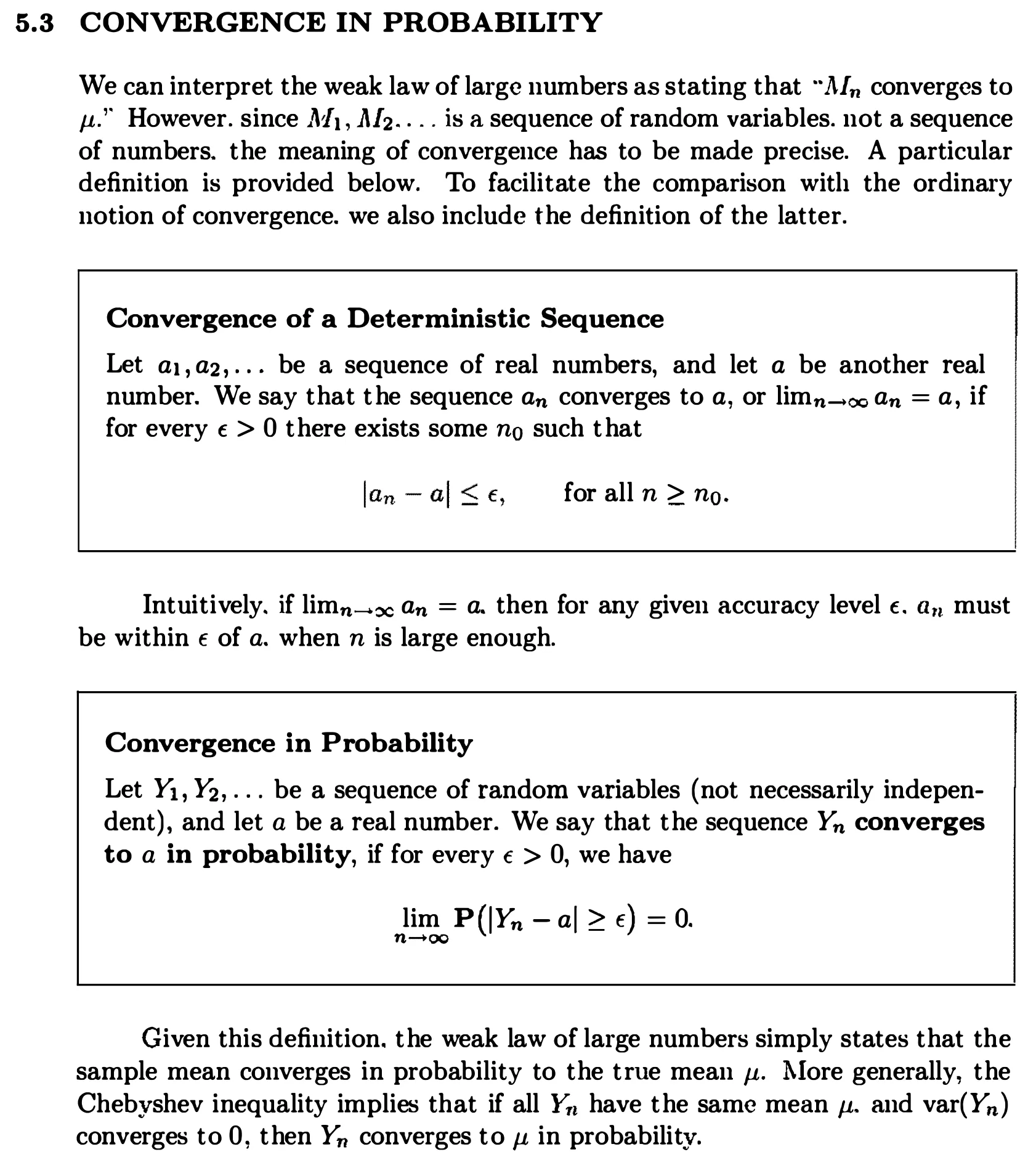
CONVERGENCE IN PROBABILITY
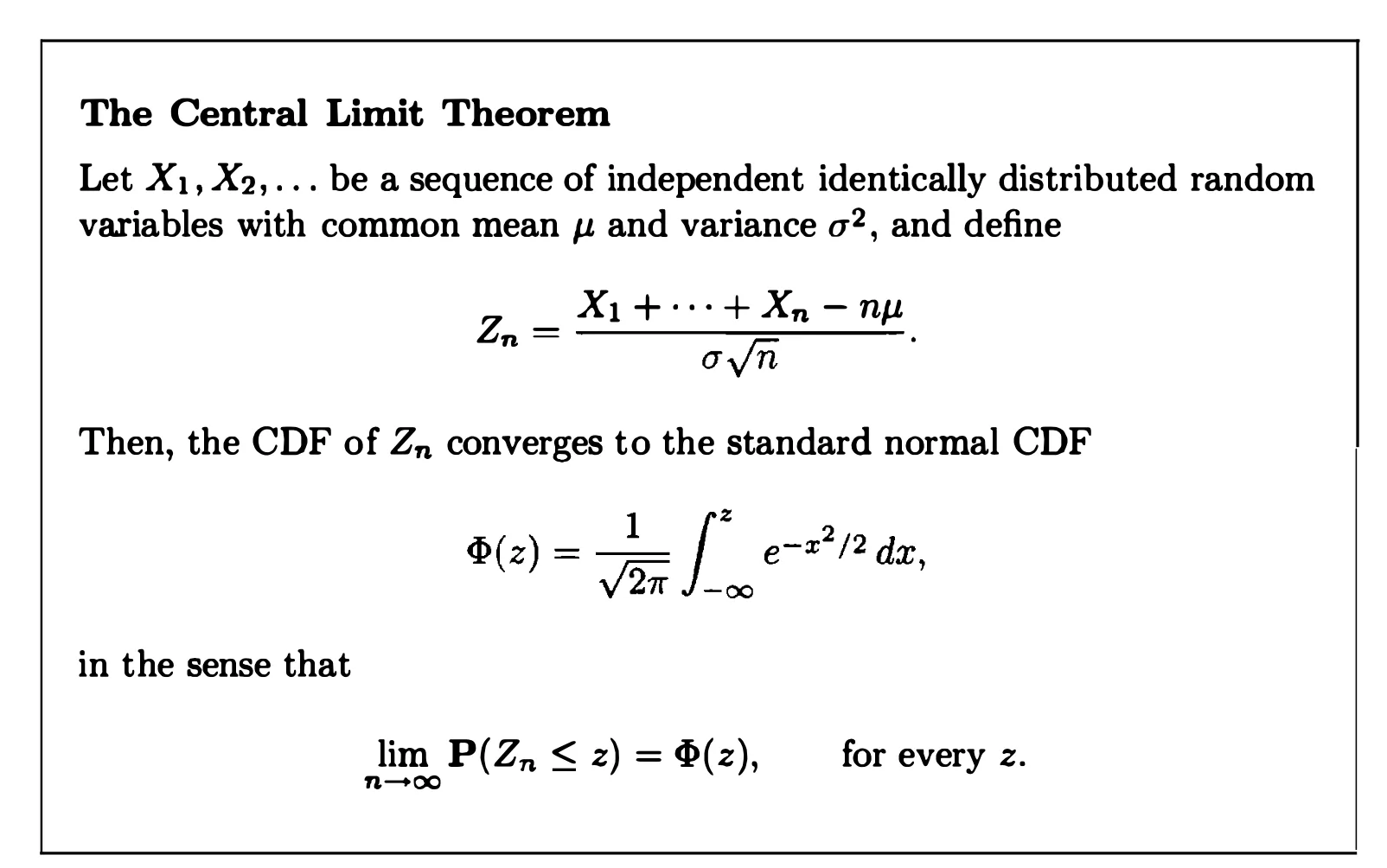
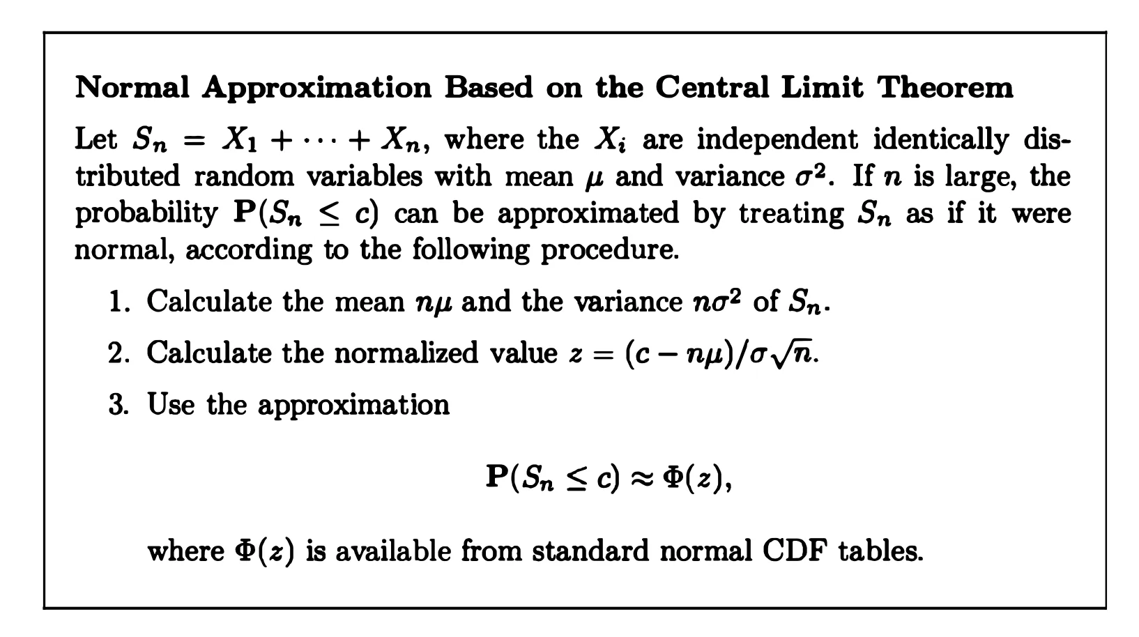
THE CENTRAL LIMIT THEOREM
It indicates that the sum of a large number of independent random variables is approximately normal. The central limit theorem finds many applications: it is one of the principal tools of statistical analysis and also justifies the use of normal random variables in modeling a wide array of situations
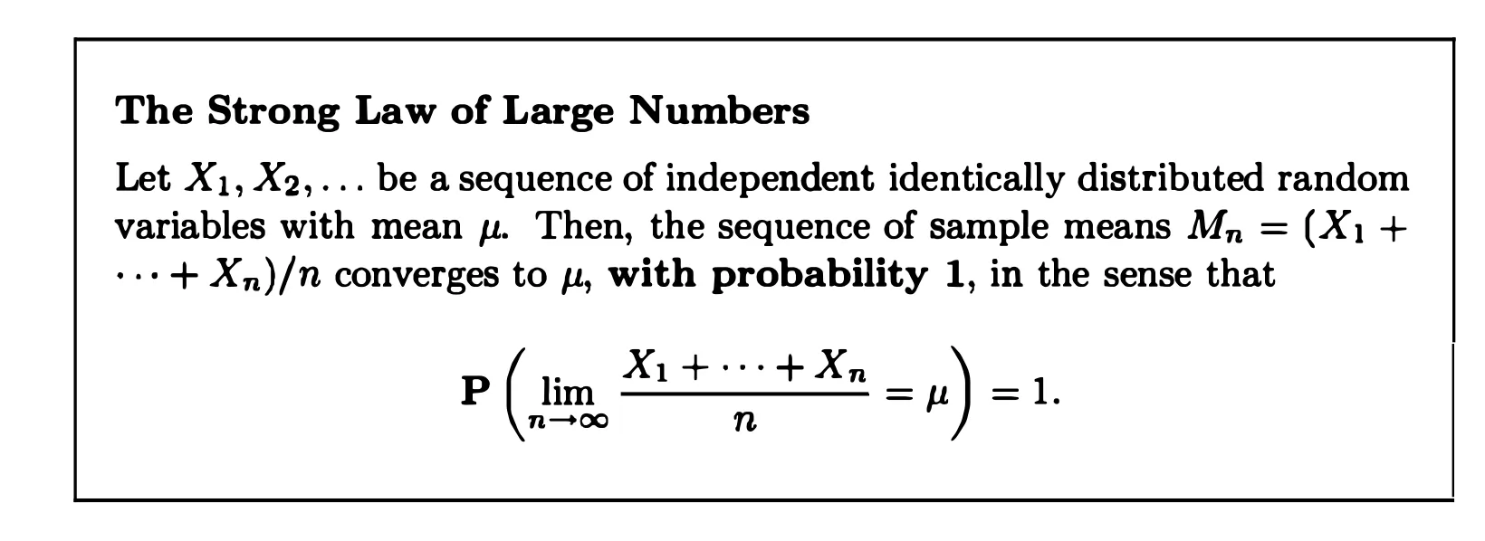
THE STRONG LAW OF LARGE NUMBERS
The Bernoulli and Poisson Processes
A stochastic process is a mathematical model of a probabilistic experiment that evolves in time and generates a sequence of numerical values.
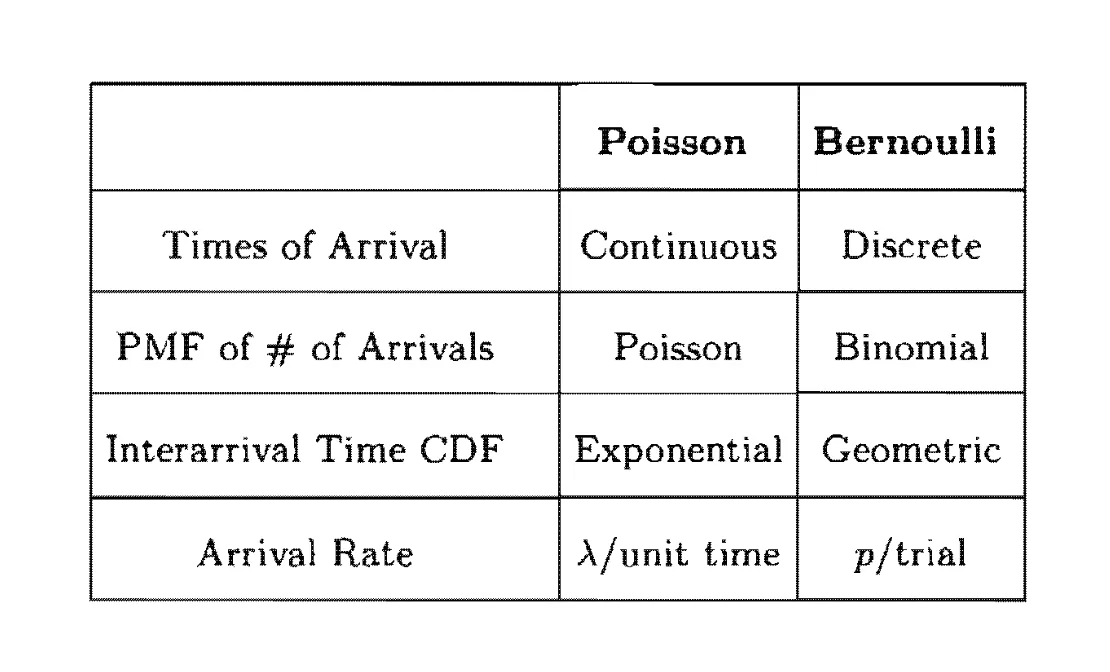
In Section 6.1, we consider the case where arrivals occur in discrete time and the interarrival times are geometrically distributed - this is the Bernoulli process. In Section 6.2, we consider the case where arrivals occur in continuous time and the interarrival times are exponentially distributed - this is the Poisson process.
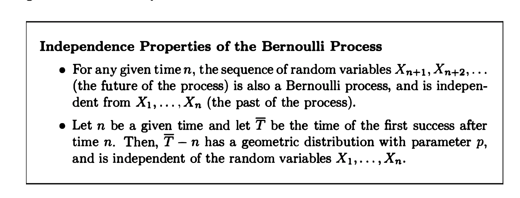
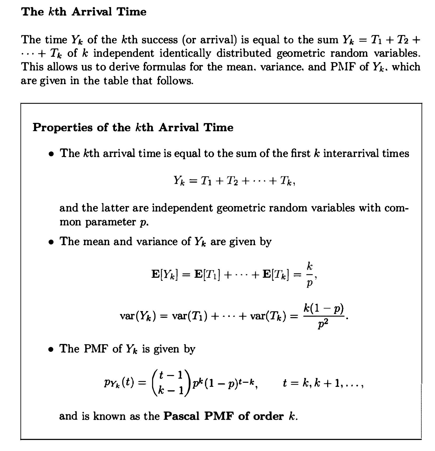
The Bernoulli Process
The Poisson Process
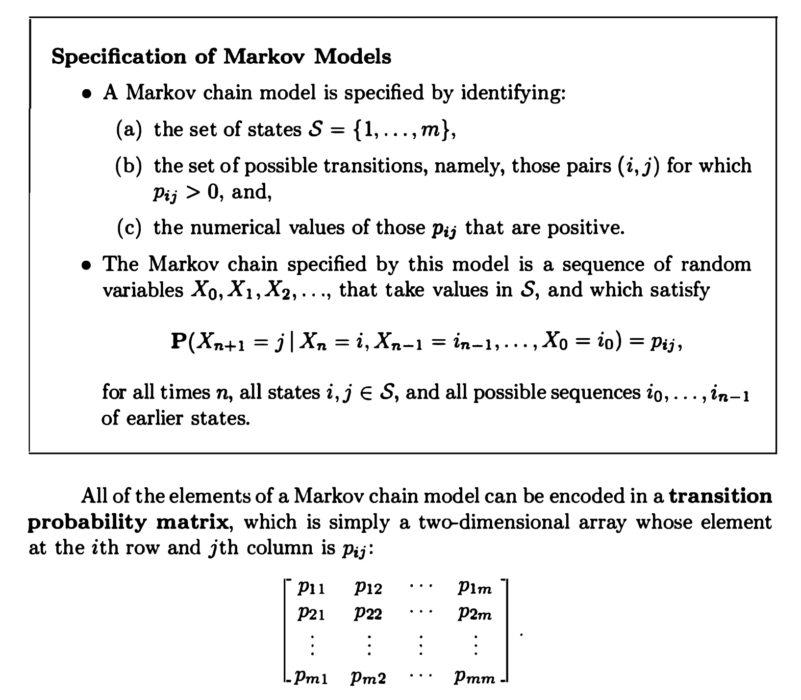
Markov Chains
Discrete-Time Markov Chains
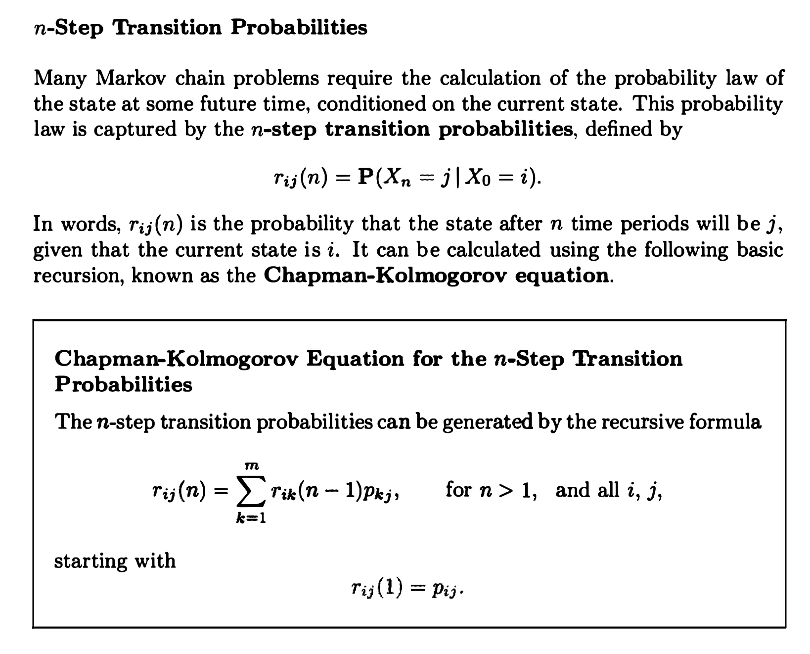
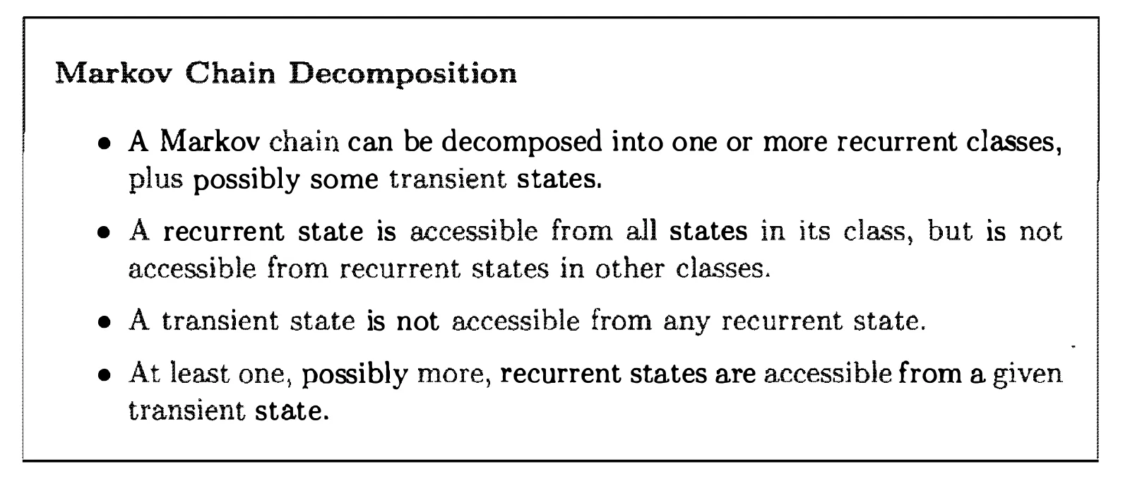
Classification of States
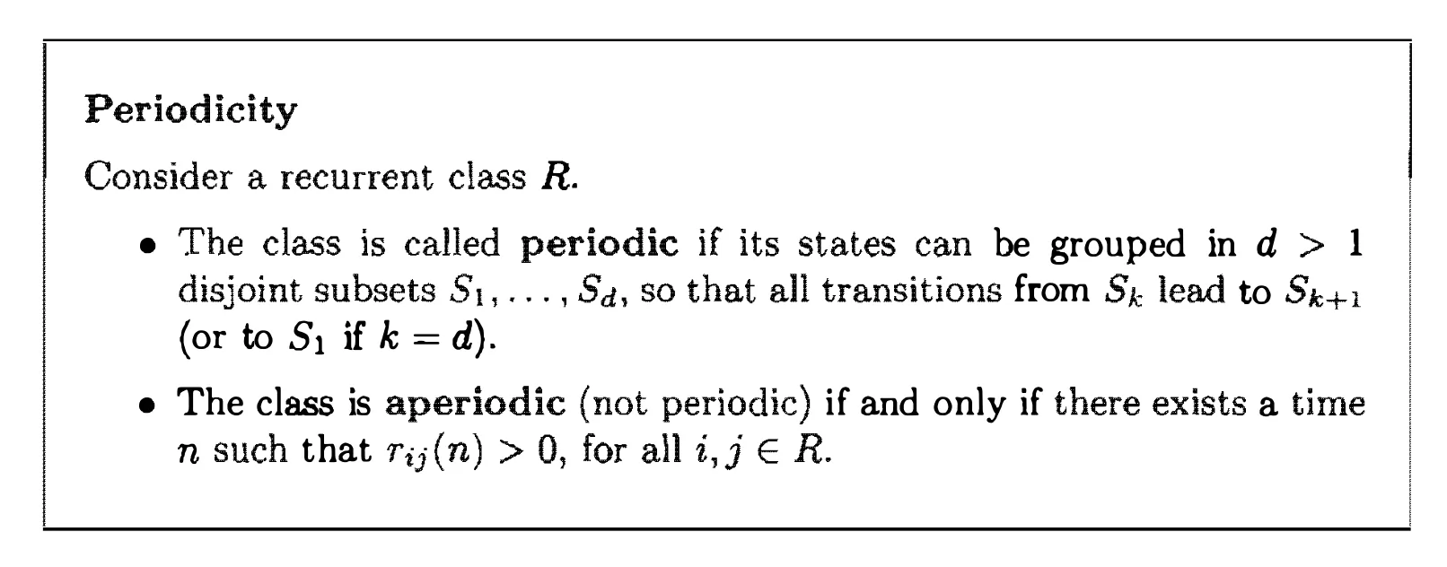
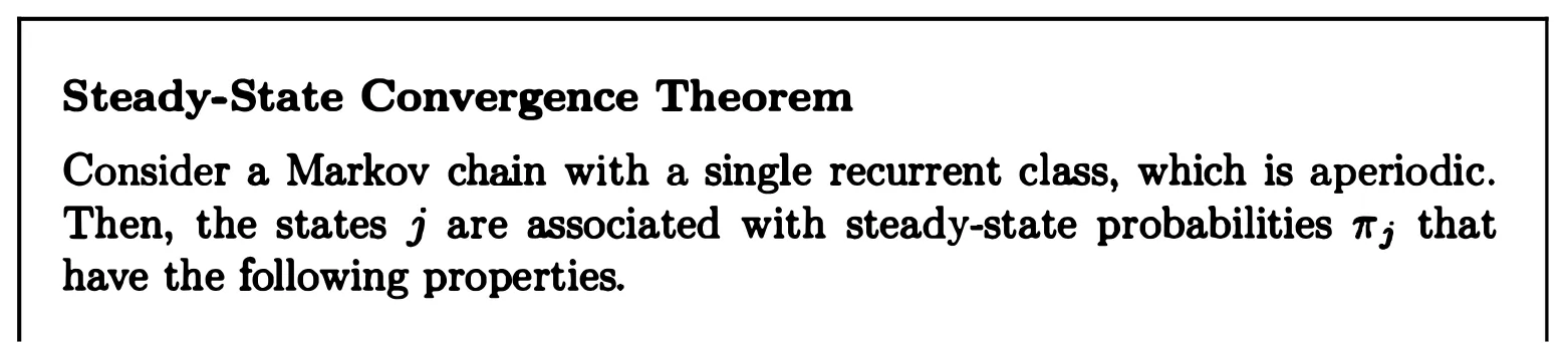
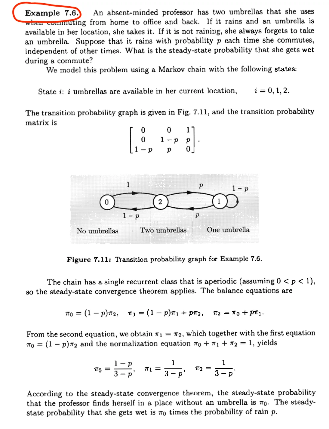
Steady-State Behavior

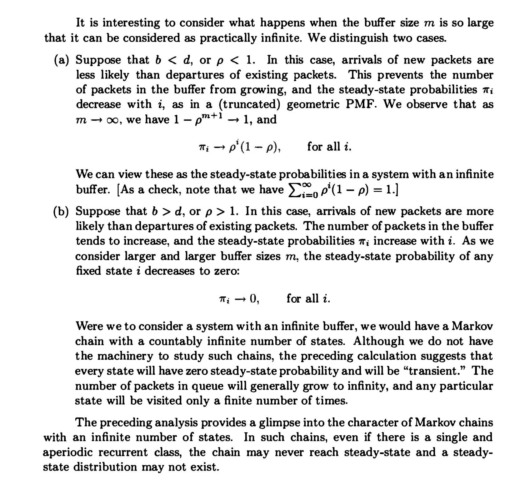
 Queueing:
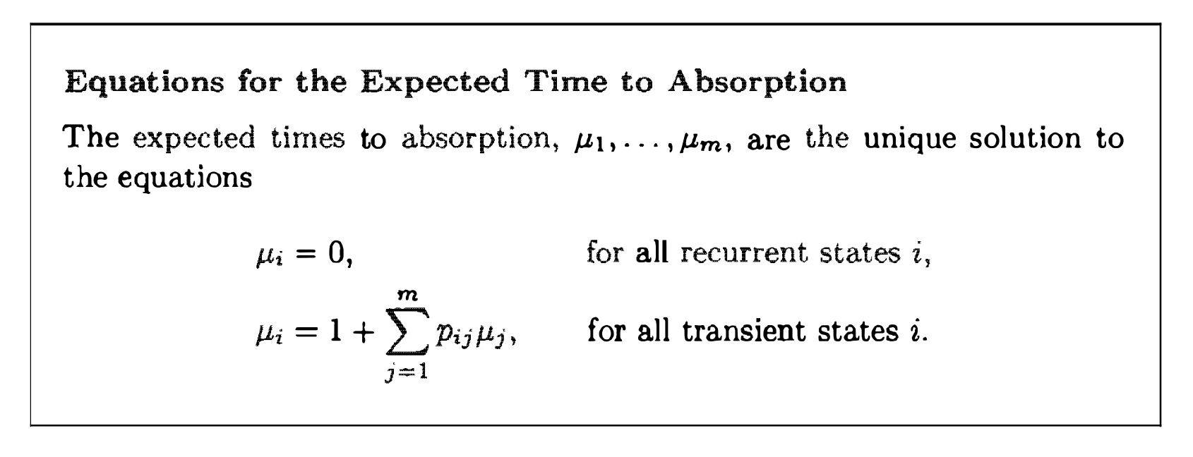
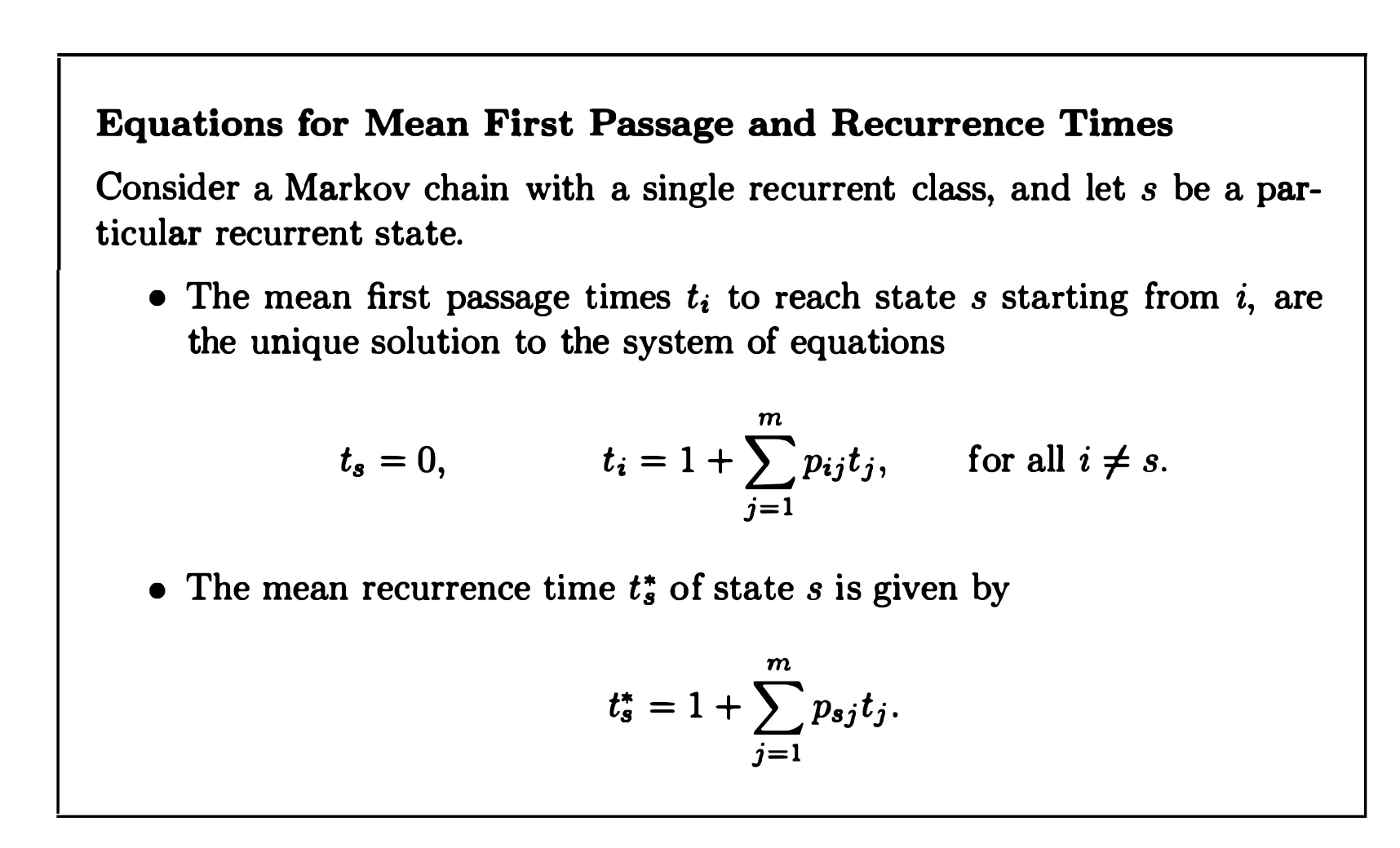
Absorption Probabilities and Expected Time to Absorption
Continuous-Time Markov Chains

Bayesian Statistical Inference
Bayesian Inference and the Posterior Distribution
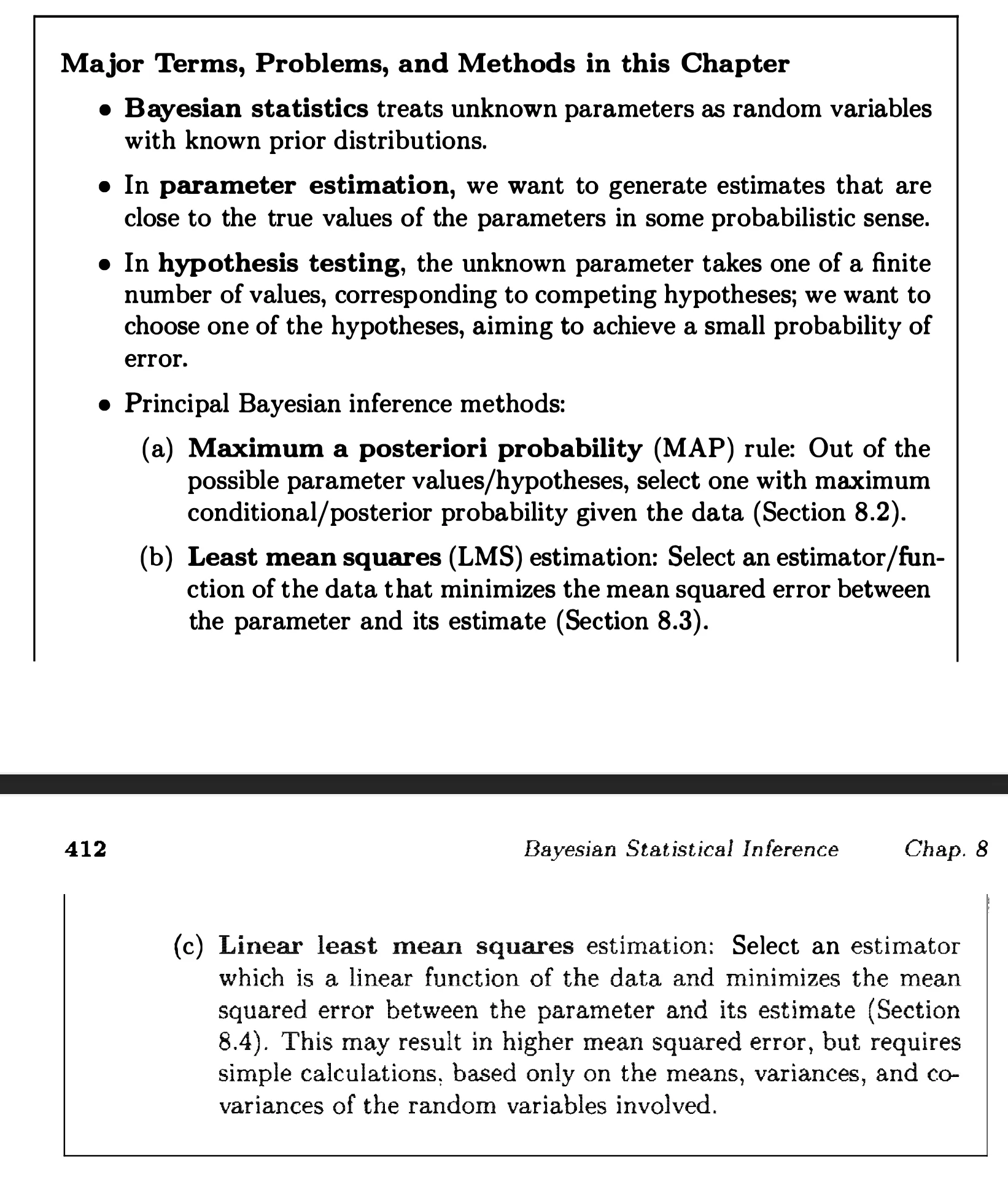
Point Estimation, Hypothesis Testing, and the MAP Rule
Bayesian Least Mean Squares Estimation
Bayesian Linear Least Mean Squares Estimation
Classical Statistical Inference
Classical Parameter Estimation
Linear Regression
Binary Hypothesis Testing
Significance Testing
Tags: Statistics
Categories: Book notes
Comments