I wanted to get in more details about the structured coalescent model, here I record some notes when I read related papers.

Overview

Firstly there is a review paper on phylogeographic inference on 2010, then I will go through some papers on structured coalescent models.

Structured coalescent papers we studied here are mainly from two authors:

• Nicola F. Muller, who developed MASCOT.
• Nicola De Maio, who developed SCOTTI.

Papers

Three roads diverged? Routes to phylogeographic inference by Erik W. Bloomquist et al. on Trends in Ecology & Evolution, 2010.

This is a summative review paper on phylogeographic inference methods.

Nested clade phylogeographic analysis (NCPA), a comparative approach

• A method to integrate molecular genealogy (often a haplotype tree) and geographic information in a single framework. Its main goal is to infer historical processes that shaped the geographic distribution of genetic variation—things like range expansions, fragmentations, or isolation by distance—using only single-locus (or sometimes multi-locus) sequence data.
• The Three-Step Workflow
  • Haplotype Tree or Network Construction: You start by building a haplotype tree or haplotype network from your molecular data (e.g., DNA sequences). Various methods can be used (parsimony, statistical parsimony, median-joining, etc.).
  • Nesting Clades: Once you have the haplotype tree, you “nest” clades in a hierarchical manner:
    • The most closely related haplotypes form the first (1‐step) clade.
    • Groups of 1‐step clades form the 2‐step clade, and so on, up to the entire tree.
    • This step is somewhat subjective and follows a set of guidelines by Templeton.
  • Statistical Tests & Interpretation:
    • For each clade, you measure how broadly it is geographically distributed relative to its genetic diversity.
    • A permutation test is used to assess statistical significance (does this clade appear more geographically “spread out” than expected by chance?).
    • Finally, you use an “inference key” (a decision flowchart) to interpret patterns (e.g., “range expansion,” “isolation by distance,” “fragmentation,” etc.).
• Criticisms:
  • High False-Positive Rate
    • Multiple studies (e.g., Knowles & Maddison; Panchal & Beaumont) showed that single-locus NCPA tends to over‐detect “significant” phylogeographic patterns, suggesting many false positives.
    • One reason is that multiple clades in the nested design are tested, but the method did not adequately correct for multiple testing (Type I error accumulation).
  • Pipeline Nature & Overconfidence
    • NCPA is a sequential pipeline:
      • Build or infer a single haplotype tree.
      • Nest the clades.
      • Do a permutation test and interpret.
    • Errors or uncertainty in earlier stages (e.g., how the tree is constructed or how clades are nested) are not carried forward—thus each subsequent step can overstate confidence in the final inferences.
• Modern model-based (particularly Bayesian or coalescent) methods are now preferred, because they:
  • They Incorporate Geography More Rigorously
    • Some methods directly model migration rates or dispersal kernels in continuous or discrete space.
    • They can handle population size changes, gene flow, barriers, and other complexities.
  • They Are Statistically Formal
    • By specifying an explicit probabilistic model of evolution + geography, one can estimate parameters (e.g., migration rates, times of divergence) and compare models via likelihood or Bayesian posterior probabilities.
  • Joint Inference
    • Many modern approaches jointly infer genealogies, demographic parameters, and geographic patterns, thus avoiding the pipeline problem where each step is conditionally fixed.

Spatial diffusion approach

1. Model‐Based Spatial Diffusion
   • Unlike traditional “population‐based” spatial coalescent models, phylogenetic diffusion focuses on the ancestral history of a particular sample of molecular sequences.
   • It treats location as a trait evolving along the branches of a time‐calibrated phylogeny, using continuous‐time Markov chains (CTMC).
   • This permits a probabilistic reconstruction of when and where the ancestors of sampled sequences existed, often implemented in BEAST.
2. Discrete vs. Continuous Spatial Models
   • Discrete diffusion: Each lineage “jumps” among a set of discrete locations. It can handle many possible states (locations), but each additional location increases the number of rate parameters.
   • Continuous diffusion: Lineages move in a continuous spatial landscape (e.g., coordinates modeled via Brownian motion or more flexible “relaxed random walks”).
   • These approaches can incorporate geographical context, such as distance‐dependent dispersal or environmental barriers, and handle rate heterogeneity over the phylogeny (relaxed clock style).
3. Bayesian Statistical Framework
   • Bayesian methods naturally account for over‐parameterization by placing priors on migration rates (e.g., distance‐informed priors).
   • They can also perform Bayesian Stochastic Search Variable Selection (BSSVS) to identify only those migration rates essential to explain the data, reducing complexity.
   • This framework yields posterior distributions reflecting uncertainty in both phylogenetic and geographic estimates.
4. Advantages & Use Cases
   • More realistic than simplistic or purely heuristic (parsimony) ancestral reconstructions.
   • Accommodates uncertainty in tree topology, branch lengths, and location histories.
   • Useful in epidemiology (e.g., viral outbreaks), biogeography (e.g., island studies, animal movement), and any case where one wants to see how lineages spread over space and time.

• Overall, this spatial diffusion approach integrates time‐scaled phylogenies with spatial movement models to infer how sampled lineages have dispersed geographically. It sidesteps full “population‐based” modeling in favor of direct ancestral locations for the sequences under study, offering a flexible, Bayesian way to reconstruct spatial histories in evolutionary and epidemiological research.

Population genetics approach

• The population genetics approach to phylogeography is dominated by methods based on the structured-coalescent framework, which models evolutionary trees as random draws from population-level processes like selection, migration, population size changes, and recombination.
• 

Comparing mugration and structured coalescent (From ChatGPT):

• Mugration models treat location as a discrete trait evolving along a single phylogenetic tree via a continuous‐time Markov chain (CTMC). They do not explicitly model different populations (demes) and their internal coalescent events.
• Structured coalescent approaches like MASCOT and SCOTTI explicitly model how lineages coalesce within demes (or hosts) and migrate or transmit between demes (or hosts). They incorporate population sizes, migration (transmission) rates, and the coalescent process in each deme.

• In other words, mugration is essentially a trait-substitution model for location, whereas structured coalescent models the population-genetic process of coalescence within and between subpopulations.

  Aspect	Mugration Model	Structured Coalescent Model (e.g. MASCOT, SCOTTI)
  Level of modeling	Per‐lineage trait substitution (no explicit coalescent events in each location).	Full coalescent with population subdivision: genealogies form via coalescence within demes, migration/transmission between demes.
  Population sizes & demes	Not modeled; “location” is just a discrete character.	Each deme (or host) has an effective population size. Coalescent rates depend on deme sizes.
  Migration	A simple CTMC of jumps between states along a single phylogeny.	Migration/transmission events between demes/hosts are part of the structured coalescent process that generates genealogies.
  Inferred quantities	- Location states at ancestral nodes - Rate matrix of location changes	- Demic or host‐level coalescent parameters (population sizes) - Migration/transmission rates - Full distribution of genealogies with demic assignment for each lineage.
  Typical usage	Reconstructing discrete phylogeography: “Where did the lineages come from and how often did they move among locations?”	Understanding population structure, host–pathogen dynamics, or transmission chains with explicit coalescent modeling.

New Routes to Phylogeography: A Bayesian Structured Coalescent Approximation by Nicola De Maio et al. on PLOS Genetics, 2015.

Abstract

• In this paper, we show that inference of migration rates and root locations based on discrete trait models is extremely unreliable and sensitive to biased sampling.
• BASTA (BAyesian STructured coalescent Approximation): a approach implemented in BEAST2 that combines the accuracy of methods based on the structured coalescent with the computational efficiency required to handle more than just few populations.

Background

• Use of the discrete trait analysis (DTA), such as mugration, entails a number of assumptions that are unusual or inappropriate when applied to the migration of lineages between geographic locations, for example
  1. the relative size of subpopulations drifts over time, such that subpopulations can become lost (extinct) or fixed (the sole remaining subpopulation) instead of being constrained, e.g. by local competition,
  2. sample sizes across subpopulations are proportional to their relative size.

Methods

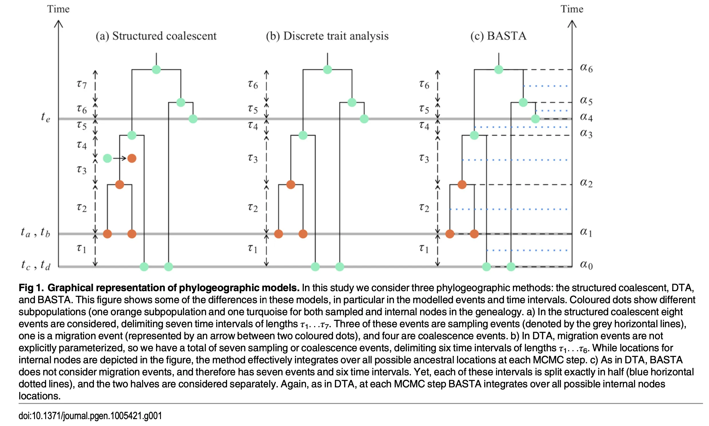
The Structured Coalescent

• Key assumptions:
  • Demes are stable in size, with their effective sizes defined by vector $\theta$.
  • Migration occurs at a constant rate over time, defined by matrix $f$.
  • No substructure within demes.
  • No fitness differences between individuals.
  • Within demes, individuals are sampled at random.
  • However, no assumptions are made about the total sample size nor the relative sample sizes per deme.
• $f_{a,b}$ is the forwards-in-time migration rate matrix, and conventionally $m_{b,a}$ is the backwards-in-time migration rate matrix. Both specifying migration of individuals from deme $a$ to deme $b$. Specifically, $m_{b,a}=f_{a,b}\theta_a/\theta_b$.

• Recall that in MultiTypeTree (MTT) for Structured coalescent:

  • The posterior distribution of the parameters is:

    \[P(T, M, \mu, m, \theta \mid S, t_I, L) \propto P(S \mid T, t_I, \mu) P(T, M \mid t_I, L, m, \theta) P(\mu) P(m) P(\theta).\]
  • Components:
    1. The first term, $P(S \mid T, t_I, \mu)$, is the likelihood of the sequences given the genealogy and substitution model, computed using Felsenstein’s pruning algorithm.
    2. The second term, $P(T, M \mid t_I, L, m, \theta)$, represents the probability density of the genealogy and migration history under the structured coalescent, given the migration matrix and effective population sizes.
    3. The third term is the prior distribution of the parameters, potentially factored as independent priors for $\mu$, $m$, and $\theta$.

  • To calculate $P(T, M \mid t_I, L, m, \theta)$, the sequence of $B$ time intervals between successive events (coalescence, sampling, or migration) is considered, starting from the most recent sample back to the root. For a haploid population:

    \[P(T, M \mid t_I, L, m, \theta) = \prod_{i=1}^B L_i,\]

    where:

    \[L_i = \exp \left[ -\tau_i \sum_{d \in D} \left( \binom{k_{i,d}}{2} \frac{1}{\theta_d} + k_{i,d} \sum_{d' \in D, d' \neq d} m_{dd'} \right) \right] E_i,\]

    and:

    • $k_{i,d}$ is the number of lineages in deme $d$ during interval $i$.
    • $E_i$ is the contribution of the event ending interval $i$:
    \[E_i = \begin{cases} 1 & \text{if it is a sampling event}, \\ m_{dd'} & \text{if it is a migration event from } d \text{ to } d', \\ \frac{1}{\theta_d} & \text{if it is a coalescence event in deme } d. \end{cases}\]

Discrete Trait Analysis

• Key Idea:
• Treats a lineage’s “location” as a discrete trait (analogous to nucleotides) evolving along an unstructured coalescent tree.
• Uses Felsenstein’s pruning algorithm to integrate over all trait histories (migration paths) very efficiently.
• Model:
• The prior on the tree often assumes a single, unstructured population.
• “Migration” is just a constant‐rate Markov chain, unrelated to actual subpopulation sizes.
• Sampling fraction $\propto$ subpopulation size is assumed.
• Pros:
• Fast and straightforward to implement (common in BEAST’s “discrete phylogeography”).
• Cons:
• Can produce biased results if real subpopulation sizes or migration strongly influence tree shape, or if sampling intensity does not match relative deme size.
  • Allows “loss” or “resurrection” of demes in unrealistic ways.
• Comparison to MTT:
  • In Discrete Trait Analysis (DTA), the migration rates do not shape the branching times or topology of the genealogy; instead, the genealogical prior is (for the most part) an unstructured coalescent (or some other simple tree prior), and “migration” is just treated as a discrete‐character substitution process on that fixed genealogy.

  • Hence, in DTA: \(P(T,\mu,f,\theta \;\big|\; S,t_I,L) \;\;\propto\;\; \underbrace{P(L \mid T, t_I, f)}_{\substack{\text{location-likelihood via discrete}\\\text{trait (migration) “substitutions”}}} \; \times \underbrace{P(S \mid T, t_I, \mu)}_{\substack{\text{sequence-likelihood via}\\\text{molecular substitutions}}} \; \times \underbrace{P(T \mid t_I,\theta)}_{\substack{\text{unstructured coalescent}\\\text{prior on the tree}}} \; \times P(\mu,f,\theta),\)

    the “tree prior” $\smash{P(T\mid t_I,\theta)}$ does not depend on the migration parameters $f$.

  • By contrast, in a MultiTypeTree (MTT) or structured coalescent model, migration does directly affect the genealogy: if lineages in the same deme coalesce faster, or if migration rates are low, that changes how quickly lineages coalesce and thus reshapes the branching pattern and times of the tree.

  • So in MTT (structured coalescent):

    \(P(T, M, \mu, m, \theta \;\big|\; S,t_I,L) \;\;\propto\;\; \underbrace{P(S \mid T, t_I, \mu)}_{\text{sequence-likelihood}} \; \times \underbrace{P(T, M \mid t_I,L,m,\theta)}_{\substack{\text{structured coalescent prior}\\\text{(tree \textit{and} migration events)}}} \; \times P(\mu)\,P(m)\,P(\theta),\) the genealogical prior $\smash{P(T,M\mid t_I,L,m,\theta)}$ does depend on $m$ (migration rates) and $\theta$, because migration directly changes how/when lineages coalesce and how the tree is shaped.

• Again, for DTA,
  • one concern is that the assumption that sampling intensity is proportional to subpopulation size leads to biased estimates of migration rates when this assumption is not met (PMID: 22190015, PMID: 24586153).
  • Second, ignoring the population structure when calculating the probability of the coalescent tree could lead to bias or lost power. For example, when migration rates are very low, one expects very long branches close to the root. This interdependency between the shape and branch lengths of the genealogy and the migration process is ignored by DTA, which could reduce accuracy.

BASTA

• Overall:
  1. BASTA integrates over migration histories in a simpler way (treating lineages’ locations as partially independent and discretizing time in sub-intervals).
  2. BASTA still allows coalescence rates to depend on whether lineages are in the same deme (unlike DTA).
  3. Because it approximates the exact (and complex) structured‐coalescent integral, it is computationally cheaper than MTT while retaining more accuracy than DTA.

• BASTA Posterior

  \[P(T, \mu, m, \theta \mid S, t_I, L) \;\;\propto\;\; \underbrace{P(S \mid T, t_I, \mu)}_{\text{sequence likelihood}} \;\times\; \underbrace{P(T \mid t_I, L, m, \theta)}_{\substack{\text{structured coalescent} \\ \text{(approx.)}}} \;\times\; P(\mu, m, \theta).\]
  • $S$: sequence data
  • $T$: the genealogy (topology + branch lengths)
  • $\mu$: mutation/substitution parameters
  • $m$: migration rates
  • $\theta$: set of effective population sizes for each deme
  • $L$: tip locations
  • $t_I$: sampling times (if heterochronous)

• In MTT, the genealogy $T$ and the explicit migration events $M$ appear:

  \[P(T, M, \mu, m, \theta \;\mid\; S, t_I, L) \;\;\propto\;\; P(S \mid T, t_I, \mu) \;\times\; \underbrace{P(T, M \mid t_I, L, m, \theta)}_{\text{structured coalescent prior (exact)}} \;\times\; P(\mu)\,P(m)\,P(\theta).\]
  • MTT attempts to fully sample each lineage’s migration path in the genealogy, which becomes computationally expensive for large datasets or many demes.

• BASTA’s Approximation

  1. Independent Migration: By writing
  \[P(d_l = d, d_{l'} = d \mid t) \approx P(d_l = d \mid t) P(d_{l'} = d \mid t),\]

  we ignore any correlation among lineages’ locations (e.g., limited carrying capacity, correlated environment, etc.).

  1. Discrete Subintervals: Instead of integrating exactly over time, evaluations are performed at only two points (start/end) per interval, assuming probabilities are constant across each half-interval.

  2. Matrix Exponential: The update

  \[P_{l, \alpha_i} = P_{l, \alpha_{i-1}} e^{\tau_i \mathbf{m}}\]

  is standard for a continuous-time Markov chain, but applying it only at interval boundaries omits any subtle interactions that might occur mid-interval.

• Why It Makes BASTA Faster

  • Exact MTT: Must consider every possible lineage location at every moment — this grows combinatorially with number of lineages/demes.
  • BASTA:
    1. Uses matrix exponentials to update each lineage’s location probabilities over sub-intervals.
    2. Approximates that lineages migrate independently within those sub-intervals.
    3. Only updates location probabilities at discrete time points (start/end of sub-intervals), skipping continuous integration.
  • Skipping a full enumeration of migration paths drastically reduces computation. BASTA still incorporates subpopulation structure into coalescent rates (unlike DTA, which ignores it altogether).

Simulation and results

• DTA overestimates migration rates when sampling intensity does not match subpopulation size.
• DTA Under-represents Uncertainty.
• DTA have lowest accuracy in estimating root locations.

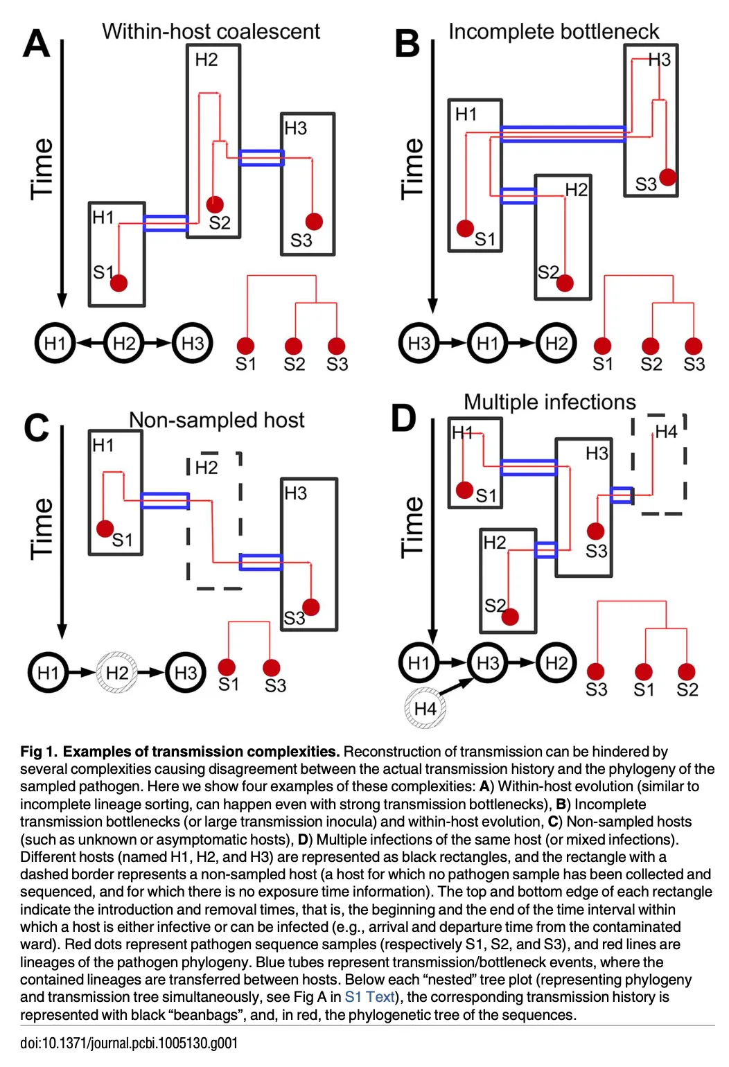
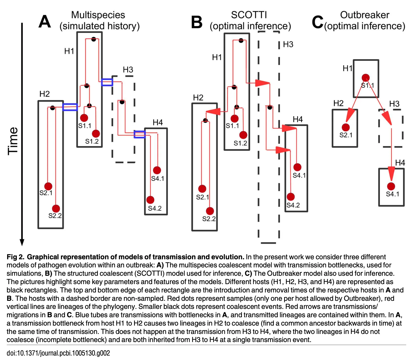
SCOTTI:Efficient Reconstruction of Transmission within Outbreaks with the Structured Coalescent by Nicola De Maio et al. on PLOS Computational Biology, 2016.

Abstract

• This study demonstrates SCOTTI (Structured COalescent Transmission Tree Inference), for modelling each host as a distinct population, and transmissions between hosts as migration events.
• Some example scenario for transmission:

Introduction

• A very good section, particularly the second and third paragraph, revisiting how others reconstruct transmission events and limitation. Should re-read sometime later.
• Outbreaker (PMID: 24465202) was compared to SCOTTI. Outbreaker did not model within-host diversity.
• One limitation of SCOTTI: do not model transmission bottlenecks.
• I found may references of this paper can be quite useful, e.g.,
  • About misleading inference if NOT modeling within-host diversity:
    • Worby CJ, Lipsitch M, Hanage WP. Within-host bacterial diversity hinders accurate reconstruction of transmission networks from genomic distance data. PLoS Comput Biol. 2014; 10:e1003549. doi: 10. 1371/journal.pcbi.1003549 PMID: 24675511
    • Romero-Severson E, Skar H, Bulla I, Albert J, Leitner T. Timing and order of transmission events is not directly reflected in a pathogen phylogeny. Molecular biology and evolution. 2014; 31(9):2472–2482. doi: 10.1093/molbev/msu179 PMID: 24874208
  • Other works considering within-host diversity, but did not considered unsampled infections:
    • Ypma RJ, van Ballegooijen WM, Wallinga J. Relating phylogenetic trees to transmission trees of infectious disease outbreaks. Genetics. 2013; 195(3):1055–1062. doi: 10.1534/genetics.113.154856 PMID: 24037268
    • Didelot X, Gardy J, Colijn C. Bayesian inference of infectious disease transmission from whole-genome sequence data. Molecular biology and evolution. 2014; 31(7):1869–1879. doi: 10.1093/molbev/msu121 PMID: 24714079
    • Hall M, Woolhouse M, Rambaut A. Epidemic reconstruction in a phylogenetics framework: transmission trees as partitions of the node set. PLoS Comput Biol. 2015; 11(12):e1004613. doi: 10.1371/journal.pcbi.1004613 PMID: 26717515
• 

Methods

• SCOTTI aims to reconstruct who infected whom and when in a scenario with multiple potential hosts (populations). This is done by:

  • Inferring a phylogeny $T$ (the genealogy of the sampled pathogen sequences).
  • Tracing how lineages “migrate” (or “transmit”) between different hosts over time.
  • Estimating parameters like:
    • Mutation/substitution parameters $\mu$ for the pathogen.
    • Migration (transmission) rate $m$ among hosts.
    • Within‐host population sizes $N_e$. ​
• The approximate structured coalescent model is based on BASTA.
  • To include the epidemiological data (host exposure time), introduction time ($d_i$) and removal time ($d_r$) were considered for each host. $[d_r, d_i]$ is the time interval when the host can host any lineage. The model assumes that $d_i$ and $d_r$ are provided for each host.
  • $\vec{E}$ is the collection of exposure times.
  • The number of hosts/populations $n_D$ is not fixed, but estimated within a specified range.
  • Migration rate $m$ is assumed the same between each pair of hosts for the time that they are both exposed to.
  • All demes have the same and constant effective population size $N_e$.
  • This means that we assume that transmission is a priori equally likely between any pair of exposed hosts, and that all hosts have equal, and constant, within-host pathogen evolution dynamics.
  • Equal population sizes and migration rates can be relaxed for known contact networks.
• Note that every sample have only one representative sequence, rather than a set of sequences representing the within-host haplotype diversity. Deep sequencing data is not utilized in this example study.

• A bit about $P_{l,\alpha_{i},d}$, the probability that lineage $l$ is in host (deme) $d$ at time $\alpha_{i}$:

  \[P_{l, \alpha_i, d} = P_{l, \alpha_{i-1}, d} \underbrace{\left( \frac{1}{D_i} + \frac{D_i - 1}{D_i} e^{-\tau_i m} \right)}_{\text{Case 1: was in } d} + \left(1 - P_{l, \alpha_{i-1}, d}\right) \underbrace{\left( \frac{1}{D_i} - \frac{1}{D_i} e^{-\tau_i m} \right)}_{\text{Case 2: was not in } d},\]

  simply adds these two scenarios:

  1. If it was already in $d$ at $\alpha_{i-1}$, the chance it stays or “effectively returns” to $d$ by $\alpha_i$.
  2. If it was not in $d$, the chance it migrates (at least once) into $d$ by $\alpha_i$.

  Notice:

  • $\frac{1}{D_i} + \frac{D_i - 1}{D_i} e^{-\tau_i m} = e^{-\tau_i m} \times 1+(1-e^{-\tau_i m})\times \frac{1}{D_i}$ = Probability of “remain in host $d$” over $\tau_i$.
  • $\frac{1}{D_i} - \frac{1}{D_i} e^{-\tau_i m} = \frac{1}{D_i}\left(1 - e^{-\tau_i m}\right)$ = Probability of “migrate from a different host into $d$” at least once.

• Simulation Setup

  1. Two Fixed Transmission Histories
     • Transmission History 1: 20 UK farms infected with FMDV in 2001 (from [15]).
     • Transmission History 2: HIV outbreak (1980–1983) involving one male index case and multiple partners (from [8]).
  2. Within-Host Coalescent Model
     • Each infected host is modeled with a constant effective population size $N_e$.
     • Lineages within a host coalesce according to a standard coalescent at rate $\tfrac{1}{N_e}$.
  3. Transmission Bottlenecks (Simulated, Not Modeled by SCOTTI/Outbreaker)
     • Weak Bottleneck ($\sim N_e$ generations of drift):
       • Two lineages have $\approx 63\%$ chance of coalescing; effectively larger fraction of the donor population survives in the recipient.
     • Strong Bottleneck ($\sim 100N_e$ generations of drift):
       • Two lineages almost surely coalesce; effectively smaller fraction of the donor population passes on.
  4. Simulation Settings
     • Factors varied:
       1. Weak vs Strong Bottleneck
       2. Transmission History 1 vs 2
       3. One vs Two Samples per Host
       4. First vs Second Transmission History (the authors label them “history 1” or “history 2”; they also mention “first vs second” might relate to repeated usage).
     • Each factor has two levels, giving $2 \times 2 \times 2 \times 2 = 8$ groups of scenarios.
  5. Further Variants per Scenario
     • For each of these 8 scenarios (“base”), they also define eight sub-scenarios (the base + 7 variants), leading to 64 distinct simulation settings:
       • Long infection: 5× longer intervals than usual ($\approx 10N_e$ generations).
       • Abundant genetic: Alignment length = 15,000 bp (instead of 1,500 bp).
       • Early sampling: Samples at 5% of the infection interval.
       • Late sampling: Samples at the end of infection.
       • Few missing: One unobserved host.
       • Many missing: Three unobserved hosts.
       • Inaccurate epi: SCOTTI is given a broader exposure interval than the true one.
  6. Number of Datasets
     • Each of the 64 scenario/variant combinations is replicated 100 times, resulting in 6,400 total simulated datasets (64 × 100).
  7. HKY Substitution Model
     • All simulations use an HKY nucleotide substitution model with:
       • $\kappa = 3 \times 10^{-3}$ substitution rate per base per $N_e$ generations (unless otherwise stated).
       • Uniform nucleotide frequencies.
     • SCOTTI and Outbreaker are both run using the HKY model for inferring the phylogeny from the simulated alignments.
  8. Methods Used for Inference
     • SCOTTI:
       • Approximates structured coalescent with possible nonsampled hosts (0–2) and runs up to $10^6$ MCMC iterations.
     • Outbreaker:
       • Also uses HKY, but typically can only handle one sample per host.

Results

• The accuracy of SCOTTI remains consistently high,with the noticeable exception of the case in which sampling occurs very early in infection.
• As we increase the within-host genetic variability, we achieve this by reducing the effect of the transmission bottleneck and increasing the within-host effective population size. We notice that the accuracy of the point estimate of SCOTTI goes remarkably down. However, calibration remains at acceptable levels.
• However, providing two samples per host increases the accuracy. This supports the idea that, if available, many sequences from each host could provide sufficient information. Deep sequencing from each host could also provide sufficient information.
• SCOTTI can investigate a dataset of 50 hosts and 2 samples per host in 1-2 hours using a single processor.

The Structured Coalescent and Its Approximations by Nicola F. Müller et al. on Molecular Biology and Evolution, 2017.

Abstract

• We present an exact numerical solution to the structured coalescent that does not require the inference of migration histories. Although this solution is computationally unfeasible for large data sets, it clarifies the assumptions of previously developed approximate methods and allows us to provide an improved approximation to the structured coalescent.

Introduction

• Mugration assumes the migration process to be independent of the tree generating process. In other words, it is assumed that the shape of a phylogeny is not in any way influenced by the migration process.
• Structured coalescent requires the state (or location) of any ancestral lineage in the phylogeny at any time to be inferred.
• Marginialization approaches (seek to marginalize over all possible migration histories by treating lineage states probabilistically instead of using MCMC based sampling) allows for the analysis of larger data sets.
  • SISCO (Volz 2012)
  • BASTA (De Maio 2015)
• ESCO is the exact structured coalescent.
  • It requires solving a number of differential equations that is proportional to the “number of different states” to the power of the “number of coexisting lineages”, $m^n$.
• MASCO is the marginal lineage states approximation of the structured coalescent.
  • Reduce the number of differential equations that have to be solved between events to the “number of states” times “number of lineages”, but ignores any correlations between lineages.
• SISCO (state independence approximation of the structured coalescent) requires the additional assumption (compared to MASCO) that the state of a lineage evolves independently of the coalescent process between events.
  • This means that changes in the probabilities of lineages being in a certain state are only dependent on the migration rates, and are completely independent of other lineages in the phylogeny.

Methods

The methods part is phenomenal, I don’t know it is because I have read so many papers on structured coalescent, or it is just well written. It clearly demonstrated how the interval probability, colaescence probability, and sampling probability are calculated, for ESCO, MASCO, and SISCO.

You shold refer back to the original paper, and the associated supplementary material, for the details.

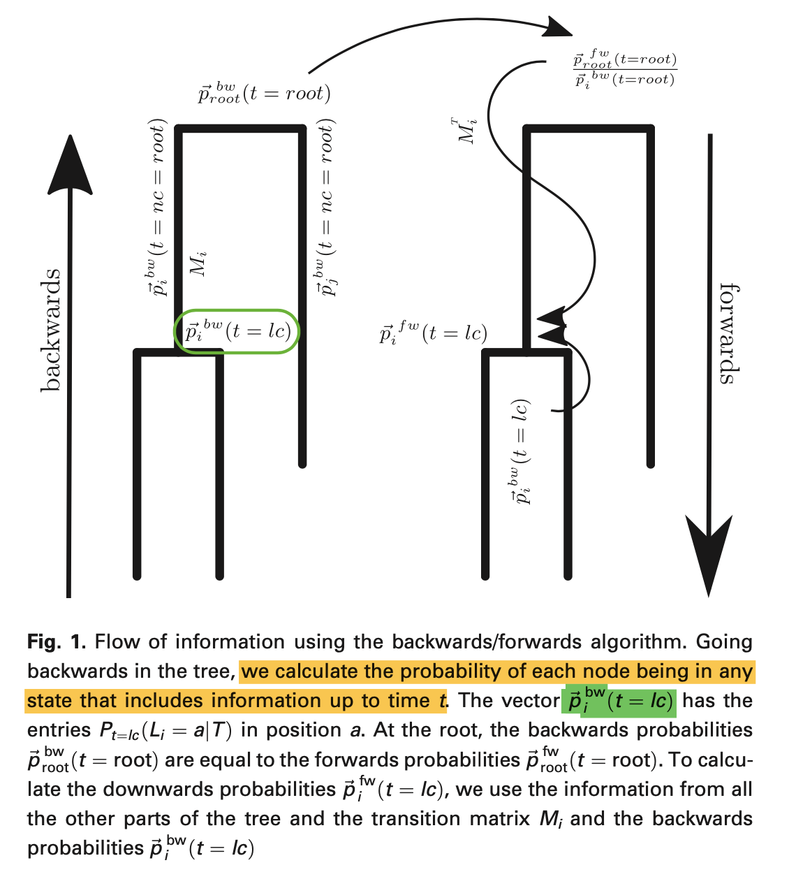
MASCOT: parameter and state inference under the marginal structured coalescent approximation by Nicola De Maio et al. on Bioinformatics, 2018.

Abstract

This study extended the previous work by calculating the probability of the state of the internal nodes of the phylogenetic tree, and now the method can handle larger datasets, including 433 H3N2 sequences from five locations.

Methods

• They used the backwards/forwards algorithm to calculate the probability of the state of the internal nodes. First going backwards in time, reaching the root, then going forwards, comparing and scaling the backwards probability for internal nodes then we get the full probability of the state of the internal nodes.
• 

Results

• With backward/forward algorithm, accuracy for internal node state probability is improved.

Discussion

• Insights for Future Studies:
  • Incorporating Explicit Sampling:
    • Future methods could explicitly incorporate sampling of migration histories or the number of state changes, using algorithms like those of Minin and Suchard (2007, 2008).
    • This would ensure probabilistic consistency with forward state probability equations.
  • Parameter Reduction:
    • Inferring all migration rates and population sizes for large datasets is computationally intensive. Strategies include:
      • Bayesian Search Variable Selection (Lemey et al., 2009): To select influential variables.
      • Generalized Linear Models (GLMs) (Lemey et al., 2014): To model migration rates based on covariates, reducing the need to infer all migration rate parameters.
  • Large datasets pose computational challenges.
    • A suggested approximation: \(\sum_{k=1, k\ne i}^n \approx \sum_{k=1}^m,\) where lineages share the same transition probabilities.
    • This approach reduces the number of ordinary differential equations (ODEs) that need to be solved.

Inferring time-dependent migration and coalescence patterns from genetic sequence and predictor data in structured populations

• MSCOT-GLM: This paper further extends the MASCOT with GLM to infer the predictors for time-varying migration rates and effective population sizes, using predictor data (like travel pattern, weekly cases).
• Similar to DTA-GLM (Lemey et al. 2014). In DTA (mugration), since the migration process is independently modelled with the coalescent process, thus the transmission dynamics in different sub-populations cannot be quantified.
• Similar to DTA-GLM, MSCOT-GLM define the migration rates, and effective population size, as log-linear combinations of coefficients, indicators and time varying predictors.

Methods

• Instead of inferring the effective population size $N_e(t)$ of state $a$ at time $t$ directly, we define it as a linear combination of $c$ different predictors $p_{N_e}(t)$, coefficients $\beta_{N_e}$, and indicators $\sigma_{N_e}$:

  \[N_e^a(t) = \beta_{N_e} \exp \left( \sum_{i=1}^c \beta_{N_e}^i \sigma_{N_e}^i p_{N_e^a}^i(t) \right).\]
• The coefficients $\beta^{i}_{N_e}$ use normal priors.
• The indicators $\sigma_{N_e}^i$ can be 0 or 1, indicating whether the predictor is used in the model.
• The number of cases when $\sigma_{N_e}^i =1$ is distributed as a given prior distribution. Typically, the prior favors a smaller number of active predictors.
• The outside $\beta_{N_e}$ is the overall scaling factor, if every indicator is $0$, then the effective population size is $\beta_{N_e}$.
• Similar for migration rates.

Results

• Seems can correctly infer the coefficients for the predictors, under simulation.
• Seems that for indicators are poorer.
• They did not showed the inffered time-varying effective population size in Figure 3, instead they only show the weekly new cases. I am curious.
• I thought that before this paper, the $N_e$ is assumed constant in MASCOT?

Discussion

• Similar GLM approaches as presented here could be applied to inform birth, death, migration, and sampling rates through time for structured birth-death models (Stadler and Bonhoeffer 2013; Kuhnert et al. 2016).

MASCOT-Skyline integrates population and migration dynamics to enhance phylogeographic reconstructions by Nicola F. Muller et al. on bioRxiv, 2024.

• The spatial and temporal transmission dynamics should be inferred simultaneously.
• MASCOT-Skyline allows us to jointly infer spatial and temporal transmission dynamics of infectious diseases using Markov chain Monte Carlo inference.
• Skyline and skygrid methods are non-parametric methods to estimate the effective population size through time.

Methods

• TODO

Results

• Nonparametric population dynamics and migration patterns can be recovered from phylogenetic trees
• Assumptions about the population dynamics drive ancestral state reconstruction in structured coalescent models
• Population structure biases population dynamic inference
• Sampling bias impacts ancestral state reconstructions
• Modeling population size dynamics is necessary to reconstruct migration rates
  • Although migration rates can be predicted using GLM (previous paper), this still relies on the models’ ability to quantify migration rates accurately.