
Course notes: Molecular Evolution workshop in Marine Biological Laboratory, US
Published: Post views:Course materials are available at here.
Day 1
Introduction to phylogenetics - Tracy Heath
- The Metazoa Phylogeny
- There is scientific controversy over whether sponges (Porifera) or ctenophores (Ctenophora) are the earliest-diverging animal lineage; traditional morphological evidence supports sponges, but some molecular studies suggest ctenophores may be more basal.
- This debate impacts our understanding of early animal evolution—especially whether complex traits like nervous systems evolved early and were later lost in sponges, or evolved independently in multiple lineages.
- Check this new evidence in Nature.
Scientific ethics - Joseph Bielawski
- Ethical reasoning focus on what I (or we) should do, but not blaming others.
- Normalization of Deviance, you should not start doing something just because it is common, or you think it has small consequences.
- Take the anti-vax movement as an example, at first it was a small group of people (deviance, Andrew Wakefield etc.), but then it became normalized and now it is a big problem.
- If you do noting, you can be contributing to normalization of deviance.
- Scientist have social privilege, and they have obligations.
Introduction to Likelihood - Paul Lewis
- Why do we need the term likelihood?
- Probability is describing the chance of an event/outcome/data given one model.
- Likelihood is describing the model/hypothesis/parameter given data.
- Transition-transversion rate ratio = 1 equivalent to transition-transversion rate = 0.5.
- Site specific rate variation, e.g. $r_1$ for codon positions 1 and 2, $r_2$ for codon position 3.
- He said that even though the parameter in the Gamma and invariable site models can have correlation, a successful bayesian search algorithm should be able to deal with this, and there are no issue with identifiability.
Model-based phylogenetics - John Huelsenbeck
- Both likelihood and distance methods can marginalize different histories along the branch (via the CTMC model).
- He revisited the Felsentein pruning algorithm.
- He explained the interpretation of the $Q$ matrix: If the process is in state $i$, we wait an exponentially distributed amount of time with parameter $-q_ii$ until the next substitution occurs; The change (after time of $e^{-q_ii}$) is $\frac{q_ij}{-q_ii}$ if the next state is $j$.
- Explained exponential distribution (waiting time for the first event), the gamma distribution (sum of exponential), the Poisson distribution (number of events in a time interval).
- One can simulate these mutations by simulating the waiting time until the next mutation, and then the change.
- You will arrive at the same result to $P(t)=e^{Qt}$. This accounts for all the ways that the process, starting in state $i$, can end up in state $j$ after time $t$.
- Note that there are two different marginalization: one is the marginalization of the history (Felsenstein), and the other is the marginalization of the multiple hits ($P(t)$).
- Stationary: if the branch length is long enough, no matter where you start, you will end up in one state with equal probability.
- We rescale the Q matrix such that the average rate of the process is $1$, then the time parameter $t$ in $P(t)=e^{Qt}$ directly represents the expected number of substitutions per site (the unit of the branch lengths). When $Q$ is scaled this way, the length of a branch ($v$) is directly interpretable as the expected number of substitutions that have occurred per site along that lineage.
Day 2
Simulating molecular evolution - John Huelsenbeck
- Transform a uniform random variable into an exponential random: $t=-\frac{ln(n)}{\lambda}$ (keeping CDF the same).
- Simulation starts from the $\pi_{A,C,G,T}$ from the root. Then we get a random number $u \in [0,1]$, and we find the first $u$ determines the root state.
- Below is an example code for simulating the state changes for v1.
- He also talked about codon model, rate variation and covarion models.
Q_matrix <- matrix(c(
  -0.886, 0.19, 0.633, 0.063,
  0.253, -0.696, 0.127, 0.316,
  1.266, 0.19, -1.519, 0.063,
  0.253, 0.949, 0.127, -1.329), nrow=4, byrow=TRUE)

mutation_matrix <-  Q_matrix
diag(mutation_matrix) <- 0
mutation_matrix <- mutation_matrix / rowSums(mutation_matrix)

v1 <- 0.3
v6 <- 0.1
v5 <- 0.1
v4 <- 0.2
v2 <- 0.1
v3 <- 0.1

# I    II   III    IV
#  \  v2 \  /v3   /
#   \     \/     /
#    \     \    /
# v1  \  v5 \  /
#      \     \/
#       \    /
#        \  / v6
#         \/

pi_vector <- c(A=0.4, C=0.3, G=0.2, T=0.1)
cumsum_pi <- cumsum(pi_vector)

(u <- runif(1))
(root_nuc_index <- max(which(u>cumsum_pi))+1)

(lambda <- -Q_matrix[nuc_index, nuc_index])

# for v1
remaining_time <- v1
current_index <- root_nuc_index
while(remaining_time > 0){
	t = -log(runif(1))/lambda
	print(t)
	# get the next event
	if(t>remaining_time){
		state_I_index <- current_index
		break
	} else{
		remaining_time <- remaining_time - t
		current_index <- sample(1:4, 1, prob=mutation_matrix[current_index,])
	}
}
print(c("A", "C", "G", "T")[state_I_index])
Model selection - David Swofford
- Models don’t need to reflect reality, but they need to be useful (think about using map vs. the real world) .
- He mentioned Felsenstein’s zone and consistency of the ML methods, compared to the Parsimony methods.
- Should we use model-based methods for phylogenetic inference when we know that assumptions about among-site rate variation and nucleotide substitution pattern are violated?
- BIC penalizes models with more parameters more strongly than AIC. BIC performs well when true model is contained in model set, and among a set of simple-ish models, AIC often selects a more complex model than the truth (indeed, AIC is formally statistically inconsistent); But in phylogenetics, no model is as complex as the truth, and the true model will never be contained in the model set; BIC often chooses models that seem too simple!; One should consider preferring AIC over BIC in phylogenetics?
- Over-partitioning: Looking closely at the estimated parameters, it is possible that one model is sufficient to explain the data.
- You can use AIC to choose the partitioning scheme, e.g., Rob Lanfear’s PartionFinder. If there are too many partitions combinations, you can use a greedy algorithm to find the best partitioning scheme.
Introduction to PAUP* - David Swofford
- PAUP* is a software package for phylogenetic analysis using parsimony and other methods (*: likelihood, and distance methods).
- Exploring Models and Hypothesis Testing using Simulation
- He confirmed an interesting point for my question: 1. when we do model selection we will need a initial tree (model), but after model selection if we choose a different model (e.g. based on AIC), the best tree may change; And changing of the best tree may further change the likelihood for model selection; that will result in a “loop”, and he confirmed that yes, we can do it iteratively.
- PAUP* can often achieve a higher likelihood than RAxML, due to fine-tuning of the optimization algorithm from Swofford.
IQ-TREE introduction
- IQ-TREE3 is now available.
- MixtureFinder is a new tool for partitioning (TODO).
- Q matrix can be customized via Qmaker or NQmaker.
- Concatenation methods for genome-scale data, and partitioned analysis.
-q,-p, and-Qare three different models for linking branch lengths. - PartitionFinder is used for merging similar partitions, to reduce calculation of considering all possible paris, clustering algorithms are used.
- Q mixture model is available (TODO).
- For species tree, gCF and sCF are useful when bootstrap supports reach 100%.
- IQ-TREE can do K-H, S-H, and AU tests, to compare trees.
- Mixture across sites and trees (MAST) model. MAST assumes that there is a collection of trees, where each site of the alignment can have a certain probability of having evolved under each of the trees. Each tree has its own topology and branch lengths, and optionally different substitution rates, different nucleotide/amino acid frequencies, and even different rate heterogeneities across sites.
IQ-TREE lab
- I like this tutorial, it looks into a real dataset, which historically caused a lot of confusion.
- Where is turtle in the tree? Different papers, different methods led to different results.
- https://doi.org/10.1186/1741-7007-10-65
- https://academic.oup.com/sysbio/article/66/4/517/2950896?login=true
- https://academic.oup.com/mbe/article/42/1/msae264/7931682?login=true
Day 3
Bayesian inference - Paul Lewis
- Joint probability, conditional probability, marginal/total probability.
- Baye’s rule: the joint probability can be written as the product of the conditional probability and the marginal/total probability: $P(A\vert B)P(B)=P(B\vert A)P(A)$.
- Note that the likelihood $L(\theta\vert D)$ is the probability of the data given the model $P(D\vert \theta)$.
- Prior can have huge impact on the posterior distribution, consider the HIV screening test example.
- A continous case: \(\underbrace{p(\theta \mid D)}_{\text{Posterior probability density}} \; = \frac{ \underbrace{p(D \mid \theta)}_{\text{Likelihood}} \;\times\; \underbrace{p(\theta)}_{\text{Prior probability density}} }{ \underbrace{\displaystyle \int p(D \mid \theta)\,p(\theta)\,\mathrm{d}\theta}_{\text{Marginal probability of the data (evidence)}} }\)
- A informative prior have low variance (not necessarily low bias), and a vague prior have high variance.
- The y-axis of a PDF is not a probability, but a probability density.
- When you use posterior ratio, you can ignore the denominator.
- Metropolis algorithm allows us to explore and characterize the posterior probability distribution $p(θ,ϕ∣D)$ without ever needing to compute the intractable denominator $P(D)$.
- A nice demonstration of the MCMC robot.
- MCMCMC is a “team effort” where different chains with different “perspectives” (temperatures) on the landscape help each other to map out the entire territory effectively. By adjusting the temperatures, we can control how the posterior distribution being flattened or sharpened, which can help us to explore the posterior distribution more efficiently.
MCMC proposals in phylogenetics - Paul Lewis
- The Largest-Simon move:
- Step 1: Pick 3 contiguous edges randomly, defining two subtrees, X and Y.
- Step 2: Shrink or grow selected 3-edge segment by a random amount.
- Step 3: Choose X or Y randomly, then reposition randomly (NNI).
- After NNI, we get a proposed tree, we will decide whether to accept basing on the log-posterior.
- While the strategy of optimizing topology and then branch lengths iteratively is key to finding a single optimal tree in ML, Bayesian MCMC aims to explore the entire landscape of possibilities. A key of the MCMC proposal is to maintain symmetricly, and making sure that the time it stays at the higher posterior region is longer than the time it stays at the lower posterior region.
- Remember that MCMC is primarily about deciding whether to accept a randomly proposed move.
- The proposal mechanism itself is generally “blind” to whether the new state will have a higher or lower posterior probability. It just generates a candidate state. The Metropolis-Hastings acceptance step then evaluates the proposed state’s posterior probability relative to the current state’s and decides whether to accept the move. This acceptance step is what guides the chain towards regions of higher posterior probability over time.
- 95% HPD interval: highest posterior density interval, the region of parameter space that contains 95% of the posterior probability mass.
- Prior distributions:
- Gamma(a, b): appropriate for parameters that range from 0 to infinity, such as branch lengths or rates.
- Lognormal: ranges from 0 to infinity, yields a paticular mean and variance.
- Beta(a,b) distributions are appropriate for proportions, which must lie between 0 and 1 (inclusive).
- A Dirichlet(a,b,c,d) distribution is ideal for nucleotide relative frequencies.
- Discrete uniform can be used for tree topologies.
- Gamma-Dirichlet can be used for branch lengths
- Gamma prior on Total Tree Length (TL), then Dirichlet Prior on Edge Length Proportions.
- It solves the problem of overestimation by default i.i.d. exponential priors (which implicitly enforce an unwanted informative prior) (the prior mean and variance of the total tree length can increase linearly with the number of taxa, sometimes leading to unrealistically long trees (“branch length overestimation”) if the data is sparse or sequences are highly similar, see Ziheng’s):
- Yule (pure birth) prior: a prior distribution that can jointly specify both the tree topology and its edge lengths.
- Check distribution explorer! https://distribution-explorer.github.io/
- Hierarchical models: some parameters of the prior distributions (called hyperparameters) are themselves drawn from another distribution (a hyperprior).
- Empirical Bayes:
- Instead of setting a hyperprior on a parameter of the prior distribution (like the mean of the branch length prior), the Empirical Bayes uses the data (e.g. MLEs) to get an estimate for this parameter.
- This approach uses the data “twice”: once to inform the prior and again in the likelihood calculation. It’s a pragmatic approach but differs from a fully Bayesian hierarchical model where all parameters, including hyperparameters, have prior distributions.
- rjMCMC: a type of Markov Chain Monte Carlo algorithm that allows the MCMC chain to jump between models of different dimensions. Useful for:
- Substitution model averaging/selection
- Species delimitation
- Marginal likelihood and Bayes factors
- The marginal likelihood is higher in models when they are true.
- Marginal likelihood inherently penalizes models that are overly complex and do not fit the data well, often favoring models that better capture the true underlying process that generated the data.
- Dirichlet process (DP) prior
- The Dirichlet Process prior is presented in the context of analyzing data from multiple loci (e.g., genes A, B, C, D) and wanting a prior that can model the situation where:
- Some loci might share the same tree topology (concordance).
- Other loci might have different tree topologies (discordance), possibly due to processes like incomplete lineage sorting.
- BUCKy model: Ané et al. 2007. Molecular Biology and Evolution 24:412–426.
- Use Concentration Parameter($\alpha$) to suggest how frequent different loci share the same tree.
- https://plewis.github.io/applets/dpp/
- The Dirichlet Process prior is presented in the context of analyzing data from multiple loci (e.g., genes A, B, C, D) and wanting a prior that can model the situation where:
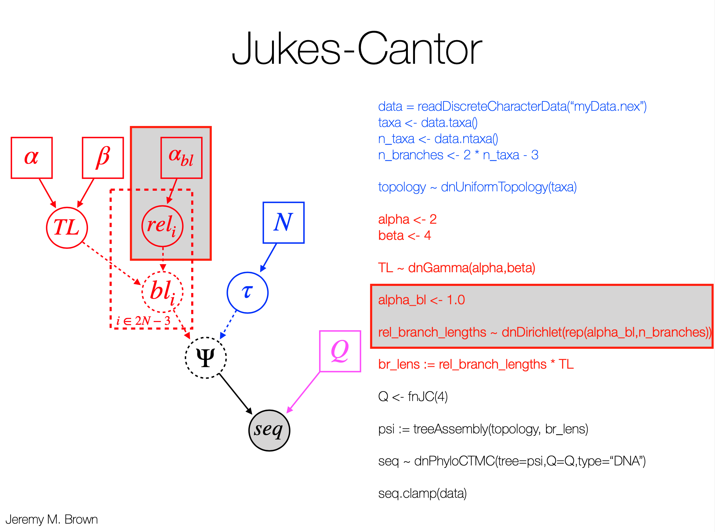
Intro. to Graphical Models and RevBayes - Jeremy Brown
- In Rev language,
z ~ dnBernoulli(0.5)is creating a random variablezwhich is fundamentally a stochastic node in the model graph. z.clamp(1)thenz.probability()will return the probability ofzbeing 1.- Graphical models provide a means of depicting the dependencies among parameters in probabilistic models.
- Squared boxes represent constant nodes:
x <- 2.3 - Dashed circles represent deterministic nodes:
y := 2 * x - Solid circles represent stochastic nodes:
z ~ dnExponential(1) - Filled solid circles represent clamped stochastic nodes:
z.clamp(1) - Plates are used to indicate replication (for loop) in the model.
- Squared boxes represent constant nodes:
- Setting up MCMC in RevBayes
- We use the
=assignment operator for “workspace” variables:myModel = model(n) - We need to define a proposal distribution (move) for any parameters we are trying to infer.
moves = VectorMoves()moves.append( mvSlide(p,delta=0.1,weight=1) ). - We need to keep track of our progress and sampled parameter values. To do that we use monitors.
monitors = VectorMonitors()monitors.append( mnScreen(printgen=1000,p) )monitors.append( mnModel(filename=“myMCMC.log", printgen=10) ) - Next we create an MCMC object.
myMCMC = mcmc(myModel,moves,monitors), and start it withmyMCMC.run(10000).
- We use the
- We tested a simple example for inferring a parameter in binomial process in RevBayes:
p ~ dnUnif(0,1)
n <- 50
k ~ dnBinomial(n,p)
k.clamp(30)
myModel = model(n)
moves = VectorMoves()
moves.append( mvSlide(p,delta=0.1,weight=1) )
monitors = VectorMonitors()
monitors.append( mnScreen(printgen=1000,p) )
monitors.append( mnModel(filename="myMCMC.log", printgen=100) )
myMCMC = mcmc(myModel,moves,monitors)
myMCMC.run(2000000)
quit()
Run it by
rb myMCMC.rb. - It is nice that he demonstrated the Gamma-Dirichlet model in RevBayes.
- There are example Rev scripts for JC, HKY, GTR, GTR+G+I available.
- The weights in moves determine the probability of different moves being selected.
- An MCMC iteration isn’t just one move; it’s typically a series of these individual parameter update attempts (each involving a proposal, likelihood calculation, and an accept/reject decision) for many, if not all, of the parameters in the model.
- Below is an example script for the GTR+G+I model:
################################################################################
#
# RevBayes Example: Bayesian inference of phylogeny using a GTR+Gamma+Inv
#                   substitution model on a single gene.
#
# authors: Sebastian Hoehna, Michael Landis, and Tracy A. Heath
#
################################################################################


### Read in sequence data for the gene
data = readDiscreteCharacterData("data/primates_and_galeopterus_cytb.nex")

# Get some useful variables from the data. We need these later on.
num_taxa <- data.ntaxa()
num_branches <- 2 * num_taxa - 3
taxa <- data.taxa()


moves    = VectorMoves()
monitors = VectorMonitors()


######################
# Substitution Model #
######################

# specify the stationary frequency parameters
pi_prior <- v(1,1,1,1)
pi ~ dnDirichlet(pi_prior)
moves.append( mvBetaSimplex(pi, weight=2) )
moves.append( mvDirichletSimplex(pi, weight=1) )


# specify the exchangeability rate parameters
er_prior <- v(1,1,1,1,1,1)
er ~ dnDirichlet(er_prior)
moves.append( mvBetaSimplex(er, weight=3) )
moves.append( mvDirichletSimplex(er, weight=1) )


# create a deterministic variable for the rate matrix, GTR
Q := fnGTR(er,pi)


#############################
# Among Site Rate Variation #
#############################

# among site rate variation, +Gamma4
alpha ~ dnUniform( 0.0, 10 )
sr := fnDiscretizeGamma( alpha, alpha, 4 )
moves.append( mvScale(alpha, weight=2.0) )


# the probability of a site being invariable, +I
p_inv ~ dnBeta(1,1)
moves.append( mvSlide(p_inv) )

##############
# Tree model #
##############

out_group = clade("Galeopterus_variegatus")
# Prior distribution on the tree topology
topology ~ dnUniformTopology(taxa, outgroup=out_group)
moves.append( mvNNI(topology, weight=num_taxa/2.0) )
moves.append( mvSPR(topology, weight=num_taxa/10.0) )

# Branch length prior
for (i in 1:num_branches) {
    bl[i] ~ dnExponential(10.0)
    moves.append( mvScale(bl[i]) )
}

TL := sum(bl)

psi := treeAssembly(topology, bl)


###################
# PhyloCTMC Model #
###################

# the sequence evolution model
seq ~ dnPhyloCTMC(tree=psi, Q=Q, siteRates=sr, type = "DNA")
seq ~ dnPhyloCTMC(tree=psi, Q=Q, siteRates=sr, pInv=p_inv, type="DNA")

# attach the data
seq.clamp(data)


############
# Analysis #
############

mymodel = model(psi)

# add monitors
monitors.append( mnScreen(printgen=100, alpha, p_inv, TL) )
monitors.append( mnFile(filename="output/primates_cytb_GTRGI.trees", printgen=10, psi) )
monitors.append( mnModel(filename="output/primates_cytb_GTRGI.log", printgen=10) )

# run the analysis
mymcmc = mcmc(mymodel, moves, monitors)
mymcmc.run(generations=20000)


# summarize output
treetrace = readTreeTrace("output/primates_cytb_GTRGI.trees", treetype="non-clock")
# and then get the MAP tree
map_tree = mapTree(treetrace,"output/primates_cytb_GTRGI_MAP.tre")


# you may want to quit RevBayes now
q()
- https://revbayes.github.io/tutorials/ctmc/
Bayesian Divergence time estimation - Tracy Heath
- The global molecular clock - Assume that the rate of evolutionary change is constant over time, for all lineages.
- However, rates of evolution vary across lineages and over time.
- Sequence data alone provide branch lengths, in the unit of expected substitutions per site. The rate and time are not identifiable by sequence data alone.
- Tree-time priors (e.g., Yule, Birth-Death) for molecular phylogenies are only informative on a relative time scale.
- $f(R, A, \Psi, \theta_R, \theta_A, \theta_s \vert D) = \frac{f(D \vert R, A, \theta_s) f(R \vert \theta_R) f(A, \Psi \vert \theta_A) f(\theta_s)}{f(D)}$
- The parameters involved are:
- $R$: A vector representing the evolutionary rates on each branch of the tree.
- $A$: A vector representing the ages of the internal nodes in the tree (divergence times).
- $\Psi$ (Psi): The tree topology (the branching pattern).
- $\theta_R$: Hyperparameters for the model of how branch rates ($R$) evolve or are distributed (e.g., parameters of a relaxed clock model).
- $\theta_A$: Hyperparameters for the tree prior, which models how topologies ($\Psi$) and node ages ($A$) arise (e.g., parameters of a birth-death process like speciation/extinction rates).
- $\theta_s$: Parameters of the substitution model describing how sequences change (e.g., GTR rates, base frequencies, gamma shape parameter for among-site rate variation).
- $D$: The observed character data (e.g., DNA or protein sequence alignment).
- $f(D \vert R, A, \theta_s)$ - The Likelihood:
- This is the probability (or probability density) of observing the sequence data $D$, given a specific tree (defined by topology $\Psi$ and node ages $A$, which together yield branch durations), the rates of evolution along each branch ($R$), and the substitution model parameters ($\theta_s$).
- Branch lengths in units of expected substitutions per site (which the likelihood calculation uses) are obtained by multiplying the rate on a branch ($R_i$) by the duration of that branch (derived from $A$ and $\Psi$).
- $f(R \vert \theta_R)$ - The Prior on Branch Rates:
- $f(A, \Psi \vert \theta_A)$ - The Joint Prior on Node Ages and Topology (The “Tree Prior”):
- $f(\theta_s)$ - The Prior on Substitution Model Parameters:
- The parameters involved are:
- Independent/Uncorrelated Rates: Lineage-specific rates are uncorrelated when the rate assigned to each branch is independently drawn from an underlying distribution (you can do it in a for loop for every branch).
- Autocorrelated Rates: closely related lineages have similar rates. The rate at a node is drawn from a distribution with a mean equal to the parent rate.
- Note that the $\mu$ in log-normal distribution is the mean of the log-transformed rates, not the mean of the rates themselves.
- The correlation between parameters in this model makes it hard for MCMC to explore the parameter space.
- Tree priors:
- The Birth-Death Process: $\lambda$ is the speciation rate, $\mu$ is the extinction rate.
- The Yule Process: $\lambda$ is the speciation rate, $\mu$ is 0.
- We also have the origin time $\phi$, and the sampling fraction $\rho$.
- Conceptual debate in fossil calibration: Calibrations as Priors vs. Calibrations as Data (Likelihoods):
- Node Calibrations as Priors: One approach is to directly treat these calibration densities as defining the prior distribution for the age of the calibrated node(s). The overall tree prior (e.g., from a birth-death process) is then conditioned on these specified node ages
- Commonly, a parametric probability distribution (e.g., Uniform, Lognormal, Gamma, Exponential) is placed on the age of an internal node. This distribution is typically offset by the age of the oldest fossil confidently assigned to that clade, effectively setting a minimum age for that node.
- While minimum age bounds from fossils are common, reliable maximum age bounds are often difficult to establish.
- Problems with multiple calibrations as priors: Rannala (2016) showed this conditional prior approach can lead to “counterintuitive topologically inconsistent realized priors” (the effective prior on tree shapes and other node ages can be strange). Dos Reis (2016) also demonstrated that this can be computationally intractable with many calibrations.
- Node Calibrations as Likelihoods (Fossil Data Likelihood): An alternative view is to treat the fossil information (e.g., fossil age $F$) as data. The probability of observing this fossil data is then expressed as a likelihood function conditional on the age of the relevant node ($t$) in the tree, $f(F\vert t,parameters)$. This approach is argued to be conceptually simpler and more easily manageable with multiple fossil calibrations.
- Common Misinterpretation: Even if the mathematical implementation of a calibration effectively treats the fossil as data (i.e., a likelihood component), it is often misinterpreted by users as directly setting the prior distribution for the node’s age. The mathematical form for $f(t\vert F)$ (a prior on node age $t$ given fossil $F$) and $f(F\vert t)$ (likelihood of fossil $F$ given node age $t$) can be identical for certain distributions (like a shifted exponential), contributing to this confusion.
- Node Calibrations as Priors: One approach is to directly treat these calibration densities as defining the prior distribution for the age of the calibrated node(s). The overall tree prior (e.g., from a birth-death process) is then conditioned on these specified node ages
- Improving Fossil Calibration:
- The goal is to use all available fossil information in a more cohesive way.
- This is achieved by recognizing that fossils are not just isolated time points but are products of the same underlying diversification (speciation, extinction, and fossilization) process that generated the extant taxa.
- The Fossilized Birth-Death (FBD) Process (by Stadler 2010)
- The FBD process is a generative model that describes the birth of new lineages (speciation, rate $λ$), the death of lineages (extinction, rate $μ$), and the recovery of fossils (fossil sampling or recovery rate, $ψ$) through time.
- It allows all relevant fossils to contribute to the analysis, not just those used to set minimum bounds on specific nodes.
- It explicitly models the processes of speciation, extinction, and fossilization.
- From fossils to phylogenies: exploring the integration of paleontological data into Bayesian phylogenetic inference
- FBD was used in a detailed penguin phylogeny with geological time, highlighting known fossils, significant paleoclimatic events, and the estimated divergence times of crown penguins, illustrating the rich evolutionary narrative that can be reconstructed (Thomas et al. Proc. Roy Soc. B 2020; Cole et al, Nature Comm. 2022; .Ksepka et al. J. Paleontology 2023)
Tutorial: Estimating a Time-Calibrated Phylogeny of Fossil and Extant Taxa using Morphological Data
- https://revbayes.github.io/tutorials/fbd_simple/
Day 4
Deep phylogenomics - Laura Eme
- Protein models of evolution
- Empirical models
- Based on alignment data.
- Typically 20*20 matrix assuming stationarity and reversibility.
- Dayhoff, JTT, WAG, LG etc.
- One can also use AIC/BIC based methods (e.g. ModelFinder) to compare empirical models.
- FreeRate model (+R): more parameters than (+G). Does not follow a parametric distribution. Not all categories will have the same number of sites.
- Model misspecification (single-matrix models) often means systematic error (LBA).
- Fully parameterized time-reversible model
- GTR: estiamte 189 rate parameters from your data.
- Mixture model
- As reflected in Wang et al. (2008) BMC Evolutionary Biology 8: 331, the simulated data does not match the real data well, suggesting that JTT+F+G is not enough.
- Standard protein substitution models: single Q matrix
- Mixture models: combine several amino-acid replacement matrices
- Can mixtured among sites, or among branches
- Standard LG+gamma: Q matrix is the same.
- LG4M: each gamma rate category gets its own Q matrix
- LG4X: each rate category gets its own Q matrix BUT rates and weights are left out of the gamma distribution assumption
- CAT: Infinite mixture model, Bayesian framework only.
- C10, C20, …, C60: approximations of the CAT model for ML.
- Complex mixture models are often hard to compute and fail to converge (by multiple chains). PMSF approximation can be useful (available in IQtree).
- Heterotachy: changing rates of evolution at sites in different parts of the tree .
- Covarion models
- Rate-shift models
- Mixture of branch-length models (GHOST in IQtree)
- Functional shifts (functional divergence)
- FD sites violate homogeneity assumption and artefactually increase branch-length (LBA).
- Try the FunDi mixture model.
- Empirical models
- Reconstructing ‘deep’ phylogenies (large-scale species trees)
- Single gene trees are not enough to resolve ‘ancient relationships’
- “Ancient” signal erased by more recent substitutions
- Improving phylogenetic signal, one way is to use multiple genes.
- Supermatrices: combining genes together
- Supertrees
- Reconciliation methods
- Minimazing potential artefacts
- Cross validation was used to test two different topologies within Obazoa are supported by different phylogenetic models: The fitted parameter values from traning set are then used to compute the likelihood of the test set: how well the test set is ‘predicted’ by the model?
- Try to eliminate ‘noisiest’ data
- Fast-evolving site removal: Check Brown et al. 2013 PRSB, they gradually remove a proportion of the fastest evolving sites (determined by the $\Gamma$ model), then they observe the topology changes, suggesting misspecified simple model (e.g. LG) gave problematic topology.
- Fast-evolving gene removal
- Fast-evolving taxon removal
- Recoding
- GFmix model: tackle compositional bias in a protein model.
- Eme is an expert on deep evolution (a LOT of Nature papers). How does LECA looks like? How do Eukaryotes relate to Asgards?
- Recoding: instead of studying all 20 aa, recode them to e.g. 4 category.
- Testing for long branch attraction: you can test different models for whether they yield even propotion of differnt topologies under simulation.
- TODO: Check the reserach context on viruses evolution, viruses tree of life, the narrow down to flu related or coronaviruses.
- Single gene trees are not enough to resolve ‘ancient relationships’
The Coalescent: Inference using trees of ‘individuals’ - Peter Beerli
- Linking population genetics (population) and phylogenetics (trees)
- Wright-Fisher model
- The number of generations for two individuals to coalesce it a Geometric distribution with expected value $2N$.
- Canning mdoel
- Moran model
- Kingman’s coalescent
- When the population size (N) is large, the discrete-generation Wright-Fisher process can be approximated by a continuous-time process.
- Scaled Coalescence Rate ($\lambda_k$) for $k$ lineages: When time is scaled appropriately (e.g., in units of $2N$ generations for diploids, or by $\Theta=4N\mu$), the rate at which any pair of $k$ lineages coalesces is: $\lambda_k = \binom{k}{2} \frac{1}{2N} = \frac{k(k-1)}{4N}$ (the other $k−2$ lineages continue into the past without coalescing in that same infinitesimal time step or generation where the first coalescence occurred.)
- Exponential waiting time with rate $\lambda_k$ for the next coalescent event.
- Probability of a Specific Genealogy ($G$) given population size $N$: Assuming each coalescence event is independent, the probability of a given genealogy (a specific tree topology and set of coalescent times $u_j$ for each interval where there were $k_j$ lineages) is the product of the probabilities of each interval: \(P(G\vert N) = \prod_{j \text{ (intervals)}} e^{-u_j \frac{k_j(k_j-1)}{4N}} \frac{k_j(k_j-1)}{4N} \times \frac{2}{k_j(k_j-1)}\) This simplifies to: \(P(G\vert N, \text{sample size } n) = \prod_{k=2}^{n} \exp\left(-u_k \frac{k(k-1)}{4N}\right) \frac{2}{4N}\) where $u_k$ is the duration of the interval when there were $k$ lineages.
- The time to the most recent common ancestor (TMRCA) has a large variance (He demonstrated this with a simulation, even under a same population size, tree shapes can be very different).
- The sample size should be much smaller than the population size
- Wright-Fisher model
- A simulator: https://phyleauxsim.github.io/coalescent/
- Genetic data and the coalescent
- Mutation introduces new alleles into a population at rate $µ$.
- $4N\mu$ can be estimated genetic variability $S$ (Summary statistics).
- Using genetic variability alone therefore does not allow to disentangle $N$ and $µ$. With multiple dated samples and known generation time we can estimate N and $µ$ independently.
- Watterson’s Estimator ($\theta_W$): Uses the number of variable sites ($S$) in a sample of $n$ individuals from a single locus: $\theta_W = \frac{S}{\sum_{i=1}^{n-1} \frac{1}{i}}$ This estimator uses a mutation rate per locus
- Bayesian Inference using the Coalescent
- Goal: Calculate $p(\text{Model Parameters } \vert \text{Data } D)$, e.g., $p(\Theta \vert D)$.
- Uses Bayes’ rule: $p(\Theta \vert D) = \frac{p(\Theta) p(D \vert \Theta)}{p(D)}$.
- Felsenstein-like Equation for Likelihood (integrating over genealogies): The likelihood of the parameters $\Theta$ given the data $D$ involves integrating over all possible genealogies $G$:
$p(D \vert \Theta) = \int_G p(G \vert \Theta) p(D \vert G) dG$
where:
- $p(G \vert \Theta)$: Probability density of a genealogy $G$ given parameters $\Theta$ (from the coalescent model).
- $p(D \vert G)$: Probability density of the data $D$ given genealogy $G$ (from the mutation model, this is the standard phylogenetic tree likelihood).
Extensions of the basic coalescent - Peter Beerli
Recap
- The probability of a specific genealogy $G$ (topology and coalescent times $u_j$ for intervals with $k_j$ lineages) given the mutation-scaled effective population size $\Theta = 4N_e\mu$ (for diploids) is:
$P(G\vert \Theta) = \prod_{j \text{ (intervals)}} e^{-u_j \frac{k_j(k_j-1)}{\Theta}} \frac{2}{\Theta}$
- This formula involves:
- Calculating the probability of waiting time $u_j$ until a coalescence: $e^{-u_j \frac{k_j(k_j-1)}{\Theta}}$ (survival probability).
- Calculating the probability density of the specific coalescence event happening: $\frac{k_j(k_j-1)}{\Theta}$ (rate of coalescence for $k_j$ lineages) multiplied by the probability of a specific pair coalescing (which is $2/(k_j(k_j-1))$, simplifying the rate term for the interval to $2/\Theta$).
- This allows calculating the probability density of a genealogy given $\Theta$.
- This formula involves:
Extensions of the Coalescent
- The basic coalescent assumes a single, constant-sized, randomly mating population. Extensions address more realistic scenarios:
- Exponential Growth Model: If population size changes exponentially, $N(t) = N_0 e^{-gt}$ (where $N_0$ is current size, $t$ is time into the past, and $g$ is growth rate towards the present). The probability of a genealogy becomes: $P(G\vert \Theta_0, g) = \prod_{j \text{ (intervals)}} e^{-(t_j - t_{j-1}) \frac{k(k-1)}{\Theta_0 e^{-gt_j}}} \frac{2}{\Theta_0 e^{-gt_j}}$ (Here, $t_j$ is the time at the end of the interval with $k$ lineages, and $\Theta_0$ is the current mutation-scaled population size).
- Skyline Plots (Random Fluctuations): Methods like Bayesian Skyline (BEAST), Skyride, Skyfish (BEAST, RevBayes) can estimate population size changes over time.
- Bottlenecks: Estimating bottlenecks depends on their severity, duration, and the amount of data (sample size, number of loci), it is HARD.
- Migration Among Populations (Structured Coalescent):
- For multiple populations, the overall rate of events (coalescence or migration) changes. For two populations (1 and 2) with $k_1$ lineages in pop 1 and $k_2$ in pop 2, the total rate of any event is: \(\text{Total Rate} = \underbrace{\frac{k_1(k_1-1)}{\Theta_1}}_{\text{coalescence in pop1}} + \underbrace{\frac{k_2(k_2-1)}{\Theta_2}}_{\text{coalescence in pop2}} + \underbrace{k_1 M_{21}}_{\text{migration 1 } \leftarrow \text{ 2}} + \underbrace{k_2 M_{12}}_{\text{migration 2 } \leftarrow \text{ 1}}\) where $M_{ij}$ is the scaled migration rate from population $j$ to $i$ (e.g., $M_{21} = 4N_1m_{21}$ if $\Theta_1=4N_1\mu$).
- Population Splitting (Divergence Models):
- Used to estimate divergence times ($\tau$), ancestral population sizes, and migration rates between diverging populations (e.g., Isolation with Migration - IM models).
- Tracing lineages backward: a lineage in population A today had an ancestor in an ancestral population B. The timing of this “population label switch” can be modeled using hazard functions (e.g., based on a Normal distribution for the divergence time).
- The resulting genealogies incorporate coalescence, migration, and population splitting events.
- More loci generally improve the precision of divergence time estimates.
Robustness and Assumptions of the Coalescent
- Sample Size ($n \ll N_e$): Kingman’s n-coalescent assumes at most two lineages merge per generation (no multiple mergers). This is a good approximation if $n \ll N_e$ (e.g., $n < \sqrt{4N_e}$ for diploids). It’s fairly robust even if this is moderately violated, as multiple mergers become very rare with large $N_e$.
- TMRCA Estimation: The Time to Most Recent Common Ancestor (TMRCA) is often robust to sample size; even small samples can yield similar TMRCA estimates to large samples. Adding more independent loci is often more beneficial than adding more individuals per locus beyond a certain point (e.g., >8 individuals ).
- Long-Term Averages: Coalescent parameter estimates represent averages over long evolutionary timescales.
- Recombination: Standard coalescent typically assumes no intra-locus recombination. Recombination means different segments of a locus can have different genealogical histories. Ignoring recombination when it’s present can bias estimates of $\Theta$ (often upwards) and migration rates (often downwards).
Mutation Models and Genetic Data in Coalescent Inference
- Confounding $N_e$ and $\mu$: Genetic diversity (e.g., number of segregating sites $S$) is primarily a function of the product $N_e\mu$ (scaled as $\Theta$). It’s hard to estimate $N_e$ and $\mu$ separately from genetic data alone without external information (like dated samples or known mutation rates per generation).
- Methods of Inference:
- Watterson’s Estimator ($\theta_W$): $\theta_W = \frac{S}{\sum_{i=1}^{n-1} (1/i)}$ (uses mutation rate per locus).
- Bayesian Inference: Calculates $p(\Theta \vert D) \propto p(\Theta) \int_G p(G\vert \Theta)p(D\vert G)dG$. The integral sums/averages over all possible genealogies ($G$) and is usually computed via MCMC.
- Types of Mutation Models for $p(D\vert G)$:
- Infinite Sites Model: Assumes every new mutation occurs at a brand new site (no multiple hits). Leads to SNP data (bi-allelic markers). Often used with Site Frequency Spectra (SFS).
- Finite Sites Models (e.g., JC69, HKY, GTR): Allow multiple hits, back mutations. Used for aligned DNA sequences.
- Site Frequency Spectrum (SFS):
- The distribution of allele frequencies in a sample. Many recent population genomic methods use the SFS, often assuming an infinite sites model.
- Challenges with SFS:
- Accommodating real data to the infinite sites model (defining ancestral alleles, handling multi-allelic sites, errors).
- SNP ascertainment bias: How SNPs are discovered can bias the SFS if not corrected.
- May be problematic for species with high diversity / large $N_e$ where the infinite sites assumption is often violated (e.g., many tri-allelic sites observed in Anopheles).
- Population divergence time estimation using individual lineage label switching
- A potential mistake in The Anopheles gambiae 1000 Genomes Consortium: Genetic diversity of the African malaria vector Anopheles gambiae. Nature, 552(7683):96–100, Dec 2017, they report very high rate for positions with $>2$ mutations.
Genomic data for evolutionary inference - Emily Jane McTavish
The talk emphasizes that while the quantity of sequence data is rapidly increasing, outstripping analytical capabilities (a point made by Jeff Thorne as early as 1991), many choices and potential pitfalls exist:
Orthology vs. Paralogy
- Distinguishing orthologs (genes diverged by speciation) from paralogs (genes diverged by duplication) is critical.
- Including unrecognized paralogs can lead to incorrect phylogenetic inferences, as demonstrated by an example of turtle phylogeny where a small number of paralogous alignments had an extraordinary influence.
- Newer “orthology-free” methods like ROADIES aim to infer species trees directly from raw genome assemblies by sampling genes, performing pairwise alignments, and iteratively estimating gene and species trees (dubious).
Speed vs. Accuracy of Phylogenetic Inference Methods
- For very large datasets (1000+ sequences), different ML tree inference software offer trade-offs:
- RAxML/ExaML: Very efficient, especially with multiple runs.
- IQ-TREE: Also fast and relatively accurate.
- FastTree: Very fast but may have trade-offs with accuracy.
- Fasttree joke: It is fast, and it is a tree.
- The presentation notes that “quick and dirty or black box methods” used for large datasets might lead to worse answers if not carefully considered.
- Newer methods like CASTER (a site-based quartet method) are very fast but their performance on complex, real-world problems needs further evaluation.
- Comments on CASTER: Direct species tree inference from whole-genome alignments: If you have to use “quick and dirty” or black box methods in order to be able to analyze large data sets - more data may result in WORSE answers.
Is the Species Tree Always What You Want?
- Different genes can have different evolutionary histories (gene trees) due to processes like incomplete lineage sorting or introgression.
- If interested in a trait controlled by one or a few genes, the species tree may not accurately describe the evolutionary history of those specific genes.
- Holistic genome approaches, like considering ancient gene linkages, can offer insights into deep evolutionary questions, such as the sister group to all other animals.
Data Processing Choices and Ascertainment Bias
- Ascertainment bias is a bias in parameter estimation or testing caused by non-random sampling of data. It is ubiquitous and can arise from how data is collected or filtered (e.g., sampling across the tree of life, volunteer surveys, studying undergraduates).
- Missing Data in RADseq: Factors like mutations at restriction sites, clustering parameters, or low coverage can cause allele drop-out. While random missing data might not be highly problematic, phylogenetically-biased missing data can mislead inference, affecting topology, branch lengths, and support values. Simply excluding sites with high missing data can bias rate estimation downwards by preferentially removing high-rate loci. There are no universal “rules-of-thumb” for handling this due to complex interactions. Investigating a range of filtering parameters is advised. The Penstemon RADseq case study shows that missing data can be phylogenetically biased, with many loci found only in one of the major clades, suggesting that analyzing clades separately or using different filtering parameters might be necessary.
- Sequencing Error: Can be problematic when true variation is rare, as errors (often singletons) can overestimate tip branch lengths. While error correction methods exist and genotype likelihoods could help, these are not always implemented in standard phylogenetic likelihood models. High coverage likely reduces the impact of sequencing error.
- TODO: Can sequencing quality data used and implemented in phylogenetic likelihood models?
- Reference Genome Choice: Mapping reads to a reference can speed up consensus sequence generation but can also introduce bias. Variant calling can be biased towards the reference base in polymorphic regions, and branch lengths can change based on reference choice. Error rates can be correlated with distance to the reference, with errors biased towards the reference base. Reference choice can even affect topology. While sequence calls may change based on the reference, overall phylogenetic conclusions might sometimes remain unaffected.
- Base call errors match the reference base 97% of the time, so the choice of reference genome can have a large impact on the phylogeny.
- A useful tutorial on Reference Bias: https://github.com/snacktavish/TreeUpdatingComparison/blob/master/TreeUpdating.md
- Free textbook: Phylogenetics in the Genomic Era
Open Tree of Life project
The Need for a Comprehensive Tree of Life
- New and improved evolutionary trees are constantly published, but even large-scale efforts often miss a significant fraction of known biodiversity (e.g., a recent plant phylogeny covering 8,000 species still missed 40% of plants).
- Taxonomy is often used as a proxy for evolutionary history, but it can be a coarse or even misleading representation.
- Researchers use taxonomy because comprehensive phylogenies are often not available for all species of interest, keep changing, or are hard to access.
Features and Functionality
- Taxonomic Integration: Users can view the lineage of any taxon within the Open Tree Taxonomy (OTT). New taxa from uploaded trees can be added and will be incorporated into future synthetic trees, with opportunities for feedback to source taxonomies.
- Synthetic Tree: A continuously updated tree that synthesizes information from the curated phylogenies and the taxonomic backbone. It visualizes phylogenetic information and areas of conflict.
- Date Estimates (DATELife):
- The main synthetic tree currently does not have inherent branch lengths because combining diverse data types (DNA, morphology, taxonomy) makes direct branch length synthesis non-obvious.
- However, the DATELife project (Sanchez-Reyes, McTavish, O’Meara, 2024) allows for the translation of date estimates from input chronograms (dated trees) onto the Open Tree synthetic topology or a user-provided tree.
- It works by matching taxa, finding congruent nodes between source chronograms and the target topology, and using median pairwise node ages to date the target tree.
Why Use Open Tree?
- Large-scale diversity assessment: Facilitates projects like PhyloNext for analyzing phylogenetic diversity of GBIF-mediated data.
- Convenience: Easily get accurate relationships and citations for arbitrary sets of species (e.g., finding the closest relative with a reference genome).
- Custom Synthesis: Users can generate custom synthetic trees for their specific taxa of interest, potentially with personalized phylogeny rankings and choice of root.
- Bird Tree Example: A synthesis phylogeny of all birds (McTavish et al., 2025) covering 87% of species, built from 321 published trees, is available A complete and dynamic tree of birds.
Day 5
Cpp session in the morning - John Huelsenbeck
- Yesterday we talked about pointers and references, and how to construct functions that take pointers and references as arguments. You can also dereference pointers to access the data they point to.
- The evolution of PRNG algorithms, Von Neumann etc.
- A USB device called TrueRNG3 on Amazon, which is a hardware random number generator that uses quantum noise to generate random numbers.
- Making arrays/vectors: the
[]operator is just dereferencing a pointer.
#include <iostream>
#include <iomanip>

int main(int argc, char* argv[] ) {

	int x[10];
	for (int i = 0; i < 10; ++i) {
		x[i] = i * 10;
		std::cout << std::setw(3) << x[i] << " " << &x[i] << "\n";
	}

	std::cout << "\n";

	int* p = &x[3];
	std::cout << "p = " << p << "\n";
	std::cout << "p's dereferenced value: " << *p << "\n";
	std::cout << "p[0] = " << p[0] << "\n";
	std::cout << "p[1] = " << p[1] << "\n"; # you can actually put a negative index here, causing out-of-bounds access

	return 0;
}
Bayesian Model Comparison with MIGRATE - Peter Beerli
Inference of parameters
- If the model of prime interest is on population dynamics (e.g., geographic structure, colonization, recurrent gene flow, past population splitting, …), the mutation model and genealogies (trees) become nuisance (we may simply integrate them).
- The primary goal in population genetics is often to infer parameters related to geographic structure, colonization, gene flow, population splitting, etc.
- Genetic data (sequence differences) are used as a proxy because detailed historical records are usually unavailable. This necessitates additional models, like mutation models and genealogical models (e.g., the coalescent).
- Inferring the posterior probability of population model parameters ($\theta$) given the data ($D$) using Bayes’ theorem, often employing MCMC: $P(\theta\vert D) = \frac{P(\theta)P(D\vert \theta)}{P(D)} = \frac{P(\theta)\int_{G}P(G\vert \theta)P(D\vert G,\mu)dG}{\int_{\theta}P(\theta)\int_{G}P(G\vert \theta)P(D\vert G,\mu)dGd\theta}$ (where $G$ is genealogy, $\mu$ is mutation model parameters).
- Beyond just reporting posteriors, we can statistically compare different demographic models.
Structured vs. Non-structured Populations
- Non-structured (single population): Free interbreeding. Variability accumulates approximately by $N \times \mu$. Highly variable populations may persist longer.
- Structured population: Interbreeding restricted to subpopulations. Variability in a subpopulation is gained via $N_{subpop} \times (m+\mu)$ (where $m$ is immigration rate). High immigration makes it behave like a single population. Structured systems can be more resistant to extinction from threats like parasites due to slowed transmission.
Bayesian Model Comparison
- Bayesian Odds Ratios: The posterior odds ratio for two models ($M_1$ vs. $M_2$) given data ($X$) is: $\frac{P(M_1\vert X)}{P(M_2\vert X)} = \frac{P(M_1)}{P(M_2)} \times \frac{P(X\vert M_1)}{P(X\vert M_2)}$ This is (Prior Odds) $\times$ (Bayes Factor).
- Bayes Factor (BF): $BF = \frac{P(X\vert M_1)}{P(X\vert M_2)}$ This is the ratio of the marginal likelihoods of the data under each model. The log Bayes Factor (LBF) is $LBF = 2 \ln(BF)$. Interpretation of LBF magnitude:
- $0 < \vert LBF\vert < 2$: No real difference
- $2 < \vert LBF\vert < 6$: Positive evidence
- $6 < \vert LBF\vert < 10$: Strong evidence
- $\vert LBF\vert > 10$: Very strong evidence
- The marginal likelihood $P(X\vert M_i)$ is the denominator $P(X)$ in the standard Bayesian posterior calculation for parameters within model $M_i$, integrated over the entire parameter space of that model.
Marginal Likelihood Calculation
- Calculating marginal likelihoods is often complicated in MCMC applications.
- The harmonic mean estimator is unreliable.
- Accurate methods include:
- Thermodynamic integration (used by MIGRATE)
- Stepping-stone integration
- Inflated Density Ratio
MIGRATE Tutorial - Peter Beerli
- MIGRATE homepage
- He actually developped a specific file format for MIGRATE.
- We learnt how to specify structured models and population split/migration models in MIGRATE.
- The model with the highest marginal likelihood (or model probability) is the best-supported model by the data.
- An example with simulated Zika virus data illustrates model comparison for population splitting and migration scenarios.
- Bayesian model selection using marginal likelihoods allows comparison of non-nested models.
- Complex biogeographic or demographic models can be compared easily.
-
specify a migration matrix for a 5-population system where population 1 and 5 are on a mainland, population 2 is an island close to 1, population 4 is close to 5, and population 3 is far out in the sea but closest to 2. ‘Close’ means reachable by rafting, and once on an island, it will be difficult to get off again.
The migration matrix should be:
    1 2 3 4 5
  1 x 0 0 0 x
  2 x x 0 0 0
  3 0 x x 0 0
  4 0 0 0 x b
  5 x 0 0 0 x
- https://molevolworkshop.github.io/faculty/beerli/migrate-tutorial-html/MIGRATEtutorial2023.html
- I found that in Tim’s MultiTypeTree paper, actually used migrate-n as a benchmark.
Multilocus phylogeography and phylogenetics - Scott Edwards
Part I: Reticulation and the Emerging Continuum
- Incomplete Lineage Sorting (ILS) / Deep Coalescence
- Genes mirror geography within Europe
- Multilocus Models in Phylogeography: population genetic parameters like population size ($\theta = 4N\mu$), divergence time ($\tau = \mu t$), and gene flow ($M = m/\mu$).
- Whole-genome Phylogeography: using whole-genome resequencing data to investigate population structure, effective migration surfaces (EEMS), and introgression using ABBA-BABA tests (Dsuite).
Part II: PhyloG2P - Macroevolution and the Origin of Phenotypic Traits
- Genomic Signatures of Trait Associations:
- Deletion/inactivation or acceleration of conserved noncoding elements (CNEEs). The neutral theory (Motoo Kimura) predicts that functionally important regions will have lower substitution rates than less important ones; thus, acceleration can suggest a change, loss, or relaxation of function.
- PhyloAcc Software Family:
- This software connects genomic and trait variation via phylogenies.
- PhyloAcc: Models rates on branches as background ($r_0=1$), conserved ($r_1 < 1$), or accelerated ($r_2 > 1$) based on a hidden state $Z_s$ for element $i$ on branch $s$. It uses a transition matrix for $Z_s$ with parameters $\alpha$ (probability of gain of conserved state) and $\beta$ (probability of loss of conserved state).
- PhyloAcc-GT (binary traits): Extends PhyloAcc to account for gene tree variation when detecting accelerations.
- PhyloAcc-C (continuous traits): Models molecular rates ($r_0, r_1, r_2$) and phenotypic rates ($\nu$, which is $\sigma^2$ scaled by $\beta_2$ or $\beta_3$) jointly, allowing estimation of the association ($log(\beta_3/\beta_2)$) between molecular acceleration and phenotypic change. An example links molecular accelerations in a CNEE with changes in longevity in mammals.
- CNEEs linked to longevity were found near genes with diverse functions.
- Case Studies (Birds):
- Tarsus Length in Birds: Four groups (penguins, kingfishers, bulbuls, swallows) show shifts to shorter tarsus length. PhyloAcc identified ~14,000 elements accelerated in short-tarsus lineages, many in ATAC-seq peaks, near genes involved in limb development pathways.
- Convergent Evolution of Flightlessness in Palaeognathae: This section highlights the long-standing debate about whether phenotypic evolution is driven more by changes in genes or gene regulation (King & Wilson 1975). It shows the phylogeny of birds including palaeognaths. Whole-genome alignments (e.g., 42 bird species using ProgressiveCactus) and analysis of different noncoding markers (UCEs, introns, CNEEs) are used. Coalescent analyses (MP-EST) using thousands of loci (CNEEs, introns, UCEs) helped resolve the position of rheas and suggested an ancient rapid radiation, potentially in the anomaly zone where the most common gene tree might not match the species tree. The study identified convergently accelerated CNEEs in ratite (flightless bird) lineages, particularly near developmental genes. ATAC-seq data further showed CNEEs in flight-related tissues active in early chick development. The combined information suggests candidate enhancers for flightlessness.
Pangenomes for Ecology and Evolution - Scott Edwards
1. Introduction to Pangenomes:
- Moving Beyond Reference-Based Genomics: Traditional genomics often relies on mapping reads to a single reference genome. Pangenomics aims to capture the entire set of genes and genomic regions found in a group of individuals or species.
- A pangenome consists of:
- Core genome: Genes present in all individuals/strains.
- Accessory/Dispensable genome: Genes present in only some individuals/strains.
2. Pangenomes in Avian Genomics - Case Study: Scrub Jays
- Context: Avian Genomes: Birds generally have small, streamlined genomes compared to other amniotes like mammals or other reptiles. However, avian genome assembly quality is improving with new sequencing technologies: Pacbio HiFi.
- Population Size Variation: PSMC and bpp analyses show a ~60-fold range in effective population size ($N_e$) across the scrub-jay species, with Island Scrub Jays having the smallest $N_e$ and Woodhouse’s having the largest.
- Repeat Content: RepeatMasker analysis indicates over 25% repeats and transposable elements in scrub-jay genomes. There’s interspecific variation in repeat content, especially LTR elements and satellites. Male birds (ZZ) show higher counts of a specific 18-kb satellite unit.
- Genome Size Variation: Island Scrub Jay assemblies are ~100 Mb smaller than Woodhouse’s Scrub Jay. Genomescope estimates of maximum genome size vary across individuals and species.
- Telomeres: Telomeres are mentioned as barometers of age and stress, with chronic malaria shown to accelerate telomere degradation in wild birds (Ashgar et al. 2015). A recent study (Brown et al. 2024) suggests that species with smaller $N_e$ (like the Island Scrub Jay) are predicted to have shorter telomeres and show changes in the genomic proportion of telomeric sequence.
3. Pangenome Graphs and Structural Variation (SV)
- Pangenome Graphs: These graphs capture structural variation (SVs) within and between species.
- Graph “depth” (how many haplotypes cover a region) can reveal different genomic features:
- Medium depth: Normal regions.
- Low depth: SNPs or small indels.
- High depth: Large SVs, satellites, repeats.
- Graph “depth” (how many haplotypes cover a region) can reveal different genomic features:
- SVs and Population Size:
- The number of SVs scales with population size.
- The Nearly Neutral Theory of molecular evolution (Tomoko Ohta) is invoked, suggesting that the efficacy of selection depends on $N_e s$ (effective population size × selection coefficient).
- In smaller populations (like the Island Scrub Jay), slightly deleterious mutations (including SVs) can drift to higher frequencies or become fixed more easily.
- Data suggests SVs are, on average, more deleterious than SNPs. Longer SVs appear to rise to higher frequencies in the small Island Scrub Jay population.
- Inversions: Inversions are common and their numbers also track population size. Pangenome and reference-based methods can identify numerous inversions, and these inversions show enhanced differentiation ($F_{ST}$) between species.
- Copy Number Variants (CNVs) and Gene Deletions: Abundant CNVs and gene deletions are found, with patterns varying across species. Gene CNVs show a surprising pattern, with the Island Scrub Jay (smallest $N_e$) having fewer deletions but more increases in copy number compared to the larger mainland populations. These CNVs have functional consequences on gene expression (TPM - transcripts per million).
Further Reading
- Bayesian Detection of Convergent Rate Changes of Conserved Noncoding Elements on Phylogenetic Trees
- Linking sequence evolution and continuous trait data, Gemmell et al. 2024. PLoS Comp. Biol. (4): e1011995.
- TODO: The phenotypic traits for birds and avian flu evolution. Avonet database, Bayou. Can we link (serodata variations)/(DMS predictions) to accelerated rates?
Day 7
The neutral and nearly neutral theories of molecular evolution - Joseph P. Bielawski
- The fundamental evolutionary “forces” are mutation, genetic drift, and natural selection.
- Conceptual Models for Genetic Variation:
- Neo-Darwinism: Natural selection is the dominant force shaping genetic variation.
- Neutral Theory (Motoo Kimura): Genetic drift is the dominant force for most observed molecular variation and evolution.
- Nearly Neutral Theory (Tomoko Ohta): The interaction between genetic drift and selection is crucial, especially for mutations with small fitness effects.
-
Substitution: The outcome of a fixation process, representing a change in the “state” of the population at a particular genetic locus. Mutations can either be fixed or lost from a population.
- Neutral Theory of Molecular Evolution (Kimura 1968)
- Rate of Substitution ($k$): Under neutrality, the rate of nucleotide substitution ($k$) at mutation-drift equilibrium is equal to the rate of new mutations ($\mu$) per gene (or site) per generation.
- $k = (\text{new mutations}) \times (\text{probability of fixation})$
- Number of new mutations in a diploid population = $2N\mu$.
- Probability of fixation for a new neutral mutant = $1/(2N)$.
- Therefore, $k = 2N\mu \times \frac{1}{2N} = \mu$.
- Independence from Population Size: A key prediction is that the rate of neutral molecular evolution ($k$) is independent of population size ($N$). This is because in small populations, fewer new mutants arise but each has a higher chance of fixation by drift. In large populations, more mutants arise but each has a lower chance of fixation by drift.
- Molecular Clock: The constant neutral rate ($k=\mu$) implies a “molecular clock,” meaning sequences should diverge at a roughly constant rate over time.
- Functional Constraint: The evolutionary rate is inversely related to functional constraint.
- Highly functional regions have more sites where mutations are deleterious.
- Lower-rate genes/regions: More sites are functional, so more mutations are deleterious and removed by selection. The remaining (neutral) mutations contribute to $k=\mu$.
- High-rate genes/regions: More sites are neutral (less functional constraint), so a larger fraction of mutations behave neutrally and can be fixed by drift, leading to $k=\mu$.
- Distribution of Fitness Effects (DFE) under Neutral Theory:
- Lethal and strongly deleterious mutations are rapidly removed by selection and ignored by Kimura.
- Beneficial mutations are considered very rare and also ignored by Kimura.
- Neutral mutations ($s=0$, where $s$ is the selection coefficient) are considered the vast majority of mutations contributing to polymorphism and species divergence.
- Rate of Substitution ($k$): Under neutrality, the rate of nucleotide substitution ($k$) at mutation-drift equilibrium is equal to the rate of new mutations ($\mu$) per gene (or site) per generation.
- Nearly Neutral Theory (Ohta):
- Interaction of Drift and Selection: This theory emphasizes the importance of mutations with small selection coefficients (nearly neutral mutations) where both genetic drift and weak selection interact to determine their fate.
- Population Size Matters:
- The “neutral zone” (where mutations behave as effectively neutral) is defined by roughly $-1/(2N_e) < s < +1/(2N_e)$ (where $N_e$ is effective population size).
- Small populations: Have a larger “neutral space.” More mutations (including slightly deleterious ones) behave as effectively neutral and evolve by drift. Selection is less effective.
- Large populations: Have a smaller “neutral space.” Slightly deleterious mutations are more effectively eliminated by selection. Slightly beneficial mutations are fixed more frequently than by drift alone (though fixation is not certain).
- Molecular Clock Unlikely: Because the rate of evolution now depends on $N_e$ (which can change), a strict molecular clock is less likely under this theory.
- DFE under Nearly Neutral Theory:
- Includes a spectrum of slightly deleterious and slightly beneficial mutations, in addition to strictly neutral ones.
- Selective Implications / Dynamics:
- Rate slows as population becomes adapted: On a concave (saturating) fitness curve, mutations have larger fitness effects when fitness is low and smaller effects when fitness is high (closer to the optimum). This means selection is initially strong but becomes less effective as the population approaches an equilibrium.
- Population approaches an equilibrium: The phenotype may reach a steady state where mutation pressure (more ways for mutations to decrease fitness) balances selection.
- Detailed Balance: At equilibrium, the evolutionary process can reach a state of “detailed balance” where, for nearly neutral mutations, the rate of beneficial substitutions equals the rate of deleterious substitutions of the same absolute effect.
- Equilibrium phenotype is NOT necessarily the most fit: The “marginal stability” of natural proteins might not be an adaptive optimum but rather a balance. Natural selection plays a role in preventing “mutational meltdown” by purging highly deleterious mutations.
- Sometimes called “steady state models” or “balance mutation models”.
- Recommended reading for balance mutation models:
- Sella G, Hirsh AE. The application of statistical physics to evolutionary biology. Proceedings of the National Academy of Sciences. 2005. 102(27):9541-9546.
- Jones CT, Youssef N, Susko E, Bielawski JP. Shifting balance on a static mutation–selection landscape: a novel scenario of positive selection. Molecular biology and evolution. 2016. 34(2):391-407.
- Recommended reading on stability-mediated epistasis and protein evolution:
- Goldstein RA. The evolution and evolutionary consequences of marginal thermostability in proteins. Proteins: Structure, Function, and Bioinformatics. 2011. 79(5):1396-1407.
- Pollock DD, Thiltgen G, Goldstein RA. Amino acid coevolution induces an evolutionary Stokes shift. Proceedings of the National Academy of Sciences. 2012. 109(21):E1352-9.
- Index of Selection Intensity for Proteins ($d_N/d_S$ or $\omega$):
- Rationale: Proteins have a “built-in ruler” for their own neutral rate – the synonymous substitution rate ($K_S$ or $d_S$).
- Synonymous mutations do not change the amino acid sequence and are assumed to be largely selectively neutral (rate = neutral rate with respect to protein evolution).
- Non-synonymous mutations ($K_N$ or $d_N$) change the amino acid and can be deleterious, neutral, or beneficial; their rate depends on selection intensity.
- The $d_N/d_S$ ratio ($\omega$): This ratio is an index of selection intensity acting on the protein.
- $d_N/d_S < 1$: Purifying (negative) selection (most non-synonymous changes are deleterious and removed). Examples: histones.
- $d_N/d_S = 1$: Neutral evolution (non-synonymous changes are as likely to fix as synonymous ones). Examples: pseudogenes.
- $d_N/d_S > 1$: Diversifying (positive) selection (non-synonymous changes are favored and fix at a higher rate than synonymous ones). Examples: MHC, Lysin.
- This allows classification of sites or genes:
- Selectively constrained: $d_N/d_S < 1$.
- Strictly neutral: $d_N/d_S = 1$.
- Adaptive evolution: $d_N/d_S > 1$.
- Rationale: Proteins have a “built-in ruler” for their own neutral rate – the synonymous substitution rate ($K_S$ or $d_S$).
Codon Substitution Models & Analysis of Natural Selection - Joseph P. Bielawski
- Mechanistic Codon Models (Population Time-Scale) models (e.g., MutSel models) are rooted in population genetics principles, considering mutation ($\mu_{ij}$), genetic drift (effective population size $N_e$), and selection ($s_{ij}$, the selection coefficient for a change from codon $i$ to $j$ at site $h$).
- $S_{ij} = \Delta f_{ij}$ (difference in fitness between codon $j$ and $i$).
- The rate of substitution $A_{ij}^h$ from codon $i$ to $j$ at site $h$ is $\mu_{ij}N \times \frac{1}{N} = \mu_{ij}$ if $s_{ij}^h = 0$ (neutral), and $\mu_{ij}N \times \frac{s_{ij}^h}{1-e^{-Ns_{ij}^h}}$ otherwise (note that $y=\frac{s_{ij}^h}{1-e^{-Ns_{ij}^h}}$ approaches $\frac{1}{N}$ as $s_{ij} \to 0$; $y\to s_{ij}$ as $s_{ij} \to \infty$; $y \to 0$ as $s_{ij} \to -\infty$).
- Usually too complex to fit such model to real data.
- Phenomenological Codon Models (Macroevolutionary Time-Scale) models (often called “$d_N/d_S$” or “$\omega$” models, e.g., GY94) typically do not explicitly model population genetic processes but describe the overall pattern of codon substitution over longer evolutionary timescales.
- They use a few key phenomenological parameters:
- $\kappa$: transition/transversion rate ratio.
- $\pi_j$: equilibrium frequency of codon $j$.
- $\omega = d_N/d_S$: the ratio of non-synonymous to synonymous substitution rates. This is the primary parameter of interest for detecting selection.
- The instantaneous rate matrix $Q$ (typically $61 \times 61$ for sense codons) is defined using these few parameters. For example, the rate from codon $i$ to $j$ ($Q_{ij}$) might be:
- 0 if $i$ and $j$ differ by >1 nucleotide.
- $\pi_j$ for synonymous transversions.
- $\kappa \pi_j$ for synonymous transitions.
- $\omega \pi_j$ for non-synonymous transversions.
- $\omega \kappa \pi_j$ for non-synonymous transitions.
- These models assume $\omega$ is constant across all contexts (i.e., the effect of a non-synonymous change is scaled by the same $\omega$ regardless of the specific amino acids involved).
- Transition probabilities over time $P(t)$ are calculated as $P(v) = e^{Qv}$ (where $v$ is branch length).
- Site likelihoods $L_h$ are computed by summing over all possible ancestral codon states, and the total likelihood $L$ is the product of site likelihoods (or sum of log-likelihoods $l$).
- They use a few key phenomenological parameters:
- Bridging Timescales: The MutSel Framework:
- The “MutSel framework” (Mutation-Selection models) attempts to bridge the population genetic (mechanistic) and macroevolutionary (phenomenological) scales.
- Two ways to reconcile:
- Map fitness to equilibrium codon frequencies (Sella and Hirsh 2005): Site-specific fitness coefficients $f^h$ for each codon determine the expected stationary codon frequencies $\pi^h$ at that site.
- Expected index of selection intensity (Jones et al. 2016): The site-specific $d_N^h/d_S^h$ can be calculated from the MutSel rate matrix by comparing the expected rate of evolution with selection to the expected rate by drift alone. The $d_N/d_S = \omega$ of phenomenological models (like M0) is an analogue of this $dN/dS$ under the MutSel framework.
- Three Positive Selection Scenarios for how $\omega > 1$ (often interpreted as positive selection) can arise:
- Scenario 1: Frequency-Dependent Selection
- Arises from antagonistic co-evolution (host-pathogen, sexual conflict, molecular interactions). For example in host-pathogen arms races, where a common host genotype is targeted by pathogens, making rare host genotypes more fit.
- The fitness landscape is dynamic: the fitness of an amino acid changes depending on the context (e.g., frequency of other alleles or interacting partners).
- Under some interpretations of phenomenological codon models (like the “omega models”), the fitness values associated with amino acids at a site can effectively swap when a substitution occurs. This means that a change in the genetic state (a substitution) alters the fitness landscape for subsequent mutations. Phenomenological codon models (like M0) implicitly assume a form of frequency-dependent selection when $\omega > 1$.
- Scenario 2: Episodic Adaptation (Adaptive Peak Shift)
- Occurs due to exploitation of a new niche, lateral gene transfer, or gene duplication, leading to a shift in the fitness landscape.
- The fitness peak itself moves. Initially, the population is sub-optimal in the new environment, and selection drives it towards the new peak (a non-stationary process).
- The MutSel-ES (Episodic Selection) model tries to capture this.
- Conclusion: Episodic models “work” because $\omega > 1$ can be a consequence of the system moving towards a new fitness peak; they are sensitive to this non-stationary behavior. The estimated $\omega$ can be biased over increasing branch lengths.
- Scenario 3: Non-Adaptive Shifting Balance (Movement around a Stationary Peak)
- The fitness landscape (peak) is static, but mutation and drift can move a population off the fitness peak to less fit states.
- Selection then acts to “repair” these shifts, pushing the population back towards the peak. This involves positive selection without necessarily leading to adaptation beyond maintaining the current function.
- The $d_N^h/d_S^h$ ratio can vary depending on the current amino acid at the site. Even with purifying selection acting most of the time to maintain a site near its fitness peak, occasional shifts away from the peak followed by selective “repair” can lead to observed $d_N/d_S > 1$ for certain amino acid states when they are rare (i.e., when the site is “in the tail” of its fitness landscape).
- Conclusion: Positive selection ($d_N/d_S > 1$) can operate even on a stationary fitness peak due to this shifting balance process, mimicking an adaptive peak shift in terms of $\omega$ values.
- Heterotachy: This process, where $d_N/d_S$ at a site can change depending on the incumbent amino acid (effectively switching between low $\omega_1$ “near the peak” and high $\omega_2$ “in the tail”), is a form of heterotachy (rate-switching).
- Scenario 1: Frequency-Dependent Selection
- Common Types of Phenomenological Codon Models:
- M0 Model (Goldman & Yang 1994; Muse & Gaut 1994): Assumes one $\omega$ for all sites and all branches.
- Branch Models: Allow $\omega$ to vary among different branches of the tree (useful for detecting episodic adaptation on specific lineages).
- Site Models: Allow $\omega$ to vary among codon sites within the alignment (useful for detecting sites under selection across the tree).
- E.g., M3 (discrete model) allows sites to fall into several pre-defined $\omega$ categories (e.g., $\omega_0=0.01, \omega_1=1.0, \omega_2=2.0$) with certain proportions.
- Powerful approach for antagonistic co-evolution, where different sites may be under different selective pressures.
- Branch-Site Models: Combine features, allowing $\omega$ to vary among sites and also differently on pre-specified “foreground” branches versus “background” branches.
- Can detect positive selection affecting only a few sites on specific lineages.
- However, branch-site models cannot distinguish between episodic adaptive evolution for a novel function and non-adaptive shifting balance on a fixed peak without external information.
-
double & triple nucleotide changes is confounded with heterotachy:Phenomenological Load on Model Parameters Can Lead to False Biological Conclusions
- Phenotype-Genotype Codon Models (PhyloG2P)
- This section introduces an approach to link genomic evolution to phenotypic changes, leveraging phylogenies (“Phylogenetics is the New Genetics”).
- Phylogenetic comparative methods can be applied to genomic data.
- Phenotype + Genotype Models: Several models are cited that explicitly link phenotypic trait evolution with rates or patterns of molecular (DNA or codon) evolution.
- Jones et al. (2020) Phenotype-Genotype (P-G) Codon Model:
- Builds on the idea of heterotachy and covarion models for $d_N/d_S$ (where sites can switch between evolutionary regimes, e.g., $\omega_1$ low “near peak” and $\omega_2$ high “in tail”).
- A null model assumes $d_N/d_S$ evolution is independent of phenotype, while the P-G model allows gene evolution (specifically $d_N/d_S$ state) to depend on phenotypic changes.
- This allows for detecting adaptive molecular evolution linked to phenotypic shifts, possibly without requiring $d_N/d_S > 1$ globally.
- An important recommended reading shared privately from Bielawski: A New Comparative Framework for Estimating Selection on Synonymous Substitutions
Adaptive protein evolution: Introduction - Belinda Chang
- Experimental Methods for Studying Proteins:
- In vitro protein expression (using bacteria, yeast, insect, or mammalian cells) is crucial for obtaining large amounts of protein for functional and structural studies, and allows for site-directed mutagenesis to test evolutionary hypotheses.
- Structure determination methods:
- X-ray crystallography (can have issues with flexibility, crystallization conditions).
- NMR spectroscopy (good for solution-state and flexible proteins, but limited to smaller proteins).
- Cryo-electron microscopy (high resolution for larger complexes in a native-like state).
- Protein structure prediction: Homology modeling (e.g., MODELLER, Rosetta, SWISS-MODEL) and machine learning approaches (e.g., AlphaFold) are used, especially when experimental structures are unavailable or to predict structures ab initio. The “twilight zone” refers to sequence identity ranges where homology modeling becomes less reliable.
- Ancestral Protein Reconstruction (APR) Process (Thornton, 2004):
- Infer a phylogenetic tree and evolutionary model from aligned extant sequences.
- Reconstruct the ancestral protein sequence at a node of interest using ML or Bayesian methods (often a single point estimate with the highest probability).
- Synthesize the gene for the ancestral protein (e.g., by stepwise PCR from oligonucleotides).
- Subclone the gene, transform cells, and express the ancestral protein.
- Purify and characterize its function (e.g., enzyme activity, ligand binding).
- Considerations and Assessing Robustness:
- Most studies use a single, highest-probability ancestral sequence.
- Potential issues: violations of model assumptions (e.g., shifts in equilibrium frequencies), uncertainty in tree topology, statistical bias towards states with high equilibrium frequencies (which might bias towards more stable proteins).
- To assess robustness: consider alternate topologies/models, sample alternative ancestors from the posterior distribution, or sample “near-ancestor” sequences.
- Uncertainty in the reconstructed genotype does not always mean uncertainty in the phenotype (function). Experimental data is needed.
- Example: Uricase Evolution in Primates (Kratzer et al., 2014):
- Uricase metabolizes uric acid; its loss in humans and some other primates is linked to diseases like gout.
- APR was used to resurrect ancient primate uricases to determine when and how function was lost.
- The study traced a gradual decline in uricase activity through primate evolution, with inactivating mutations identified at specific codons.
- This addresses questions like “Thrifty genes vs. drifty genes” for the loss of function.
- Example: Paleoenvironments (EF-Tu thermostability) (Gaucher et al., 2008):
- Resurrected Elongation Factor Tu (EF-Tu) proteins from ancestral bacteria and archaea were used to infer ancient environmental temperatures.
- The thermostability ($T_m$) of modern EF-Tu correlates with the organism’s growth temperature.
- By measuring the $T_m$ of resurrected ancestral EF-Tu proteins (expressed in E. coli), researchers inferred that early bacterial ancestors were likely thermophilic (living at 60-80°C). The posterior distribution of ancestral $T_m$ values can be obtained by sampling from the posterior distribution of ancestral sequences.
- Rhodopsin Evolution and Nocturnality in Early Mammals:
- This section discusses investigating the hypothesis that early mammals lived in a nocturnal niche, which might have led to adaptive changes in rod photoreceptors (rhodopsin) for dim-light vision.
- Methodology:
- Ancestral rhodopsin sequences (Amniote, Mammalian, Therian) were reconstructed and expressed in vitro.
- Spectroscopic assays measured rhodopsin spectral tuning ($\lambda_{MAX}$) and the lifetime of the activated state ($t_{1/2}$), which relates to signal shut-off kinetics.
- Findings (Bickelmann et al., 2015): An increased lifetime ($t_{1/2}$) of activated rhodopsin was found in reconstructed mammalian and therian ancestors compared to the general amniote ancestor, suggesting adaptations for enhanced sensitivity in dim light.
- Glutamate Receptors (GPCRs):
- Briefly introduces metabotropic glutamate receptors (mGluRs) and other G protein-coupled receptors (GPCRs) involved in synaptic neurotransmission.
- Shows an example of reconstructed ancestral amino-acid-binding GPCRs (Kuang et al., 2006) to study the evolution of ligand binding and potency of different agonists[cite: 63, 66].
- Coral Pigments (GFP-like proteins):
- Illustrates using APR to study the evolution of fluorescent proteins in corals (e.g., great star coral, Ugalde et al., 2004). By reconstructing ancestral proteins, researchers can trace the spectral shifts (e.g., from green to red) and understand the molecular basis of color diversification.
Adaptive protein evolution: Detecting changes in selection - Belinda Chang
- Examples of Positive Selection Studies:
- Host-viral arms races:
- Primate TRIM5$\alpha$, Protein Kinase R (PKR).
- Potato virus Y.
- Neutrophil-mediated responses.
- Sperm-egg recognition: Abalone lysin.
- Sensory proteins: Visual pigments in various vertebrates.
- Transcription factors in development: Stem cell pluripotency.
- Host-viral arms races:
- Case Study: Primate Protein Kinase R (PKR) vs. Viral K3L:
- PKR is an antiviral protein; viral proteins like K3L try to mimic its substrate (eIF2$\alpha$) to evade it.
- Phylogenetic analysis shows PKR evolving rapidly ($dN/dS > 1$) in primates, while eIF2$\alpha$ is highly conserved. Viral K3L also shows evidence of rapid evolution ($dN/dS > 1$).
- Sites under positive selection in PKR are identified, particularly in the kinase domain, including regions that interact with viral antagonists or eIF2$\alpha$.
- Experimental work (yeast growth assays) demonstrated that specific, positively selected residues (e.g., F394L in gibbon PKR) are crucial for resistance to viral K3L, confirming an adaptive arms race.
- Beyond Random Sites Models - Clade Models (e.g., CmC by Bielawski & Yang 2004):
- These models allow the form and strength of selection ($\omega$) to vary across both the phylogeny (different clades/lineages) and among sites within the protein.
- Clade Model C (CmC), for example, allows sites to be in categories like:
- Always under purifying selection ($0 < \omega_0 < 1$) across the tree.
- Always evolving neutrally ($\omega_1 = 1$) across the tree.
- Evolving under divergent selection ($\omega_2 \neq \omega_3$) between pre-specified foreground and background clades.
- An improved null model (M2a_rel by Weadick & Chang 2012) is mentioned for testing divergent selection, where the third site class estimates a single $\omega$ across all branches.
- Case Study: Neotropical Cichlid Rhodopsin (Hauser et al. 2017):
- Hypothesis: Adaptation of rhodopsin (visual pigment) during the invasion of different light environments in Central and South America by cichlid fish.
- Clade models were used to test for divergent selection in rhodopsin associated with geography (Central vs. South America) and ecology (lacustrine vs. riverine).
- Strong evidence was found for accelerated rhodopsin divergence ($\omega = 14.0$ for 3.4% of sites) in the Central American cichlid lineage compared to the background South American lineage ($\omega = 4.5$).
- Site 83 was identified as under positive selection and showed independent N83D substitutions in Central American lineages.
- Experimental follow-up: In vitro expression and spectroscopic assays of rhodopsin variants showed that the N83D mutation (found in Central American fish) significantly altered rhodopsin function (faster retinal release kinetics, $t_{1/2}$), suggesting adaptation to increased light levels in clearer Central American streams.
- Future Directions: High-Throughput Functional Studies:
- Deep Scanning Mutagenesis: Experimental approaches to create and test large libraries of protein variants.
- Example: High-throughput rhodopsin variant libraries:
- Random mutagenesis of a rhodopsin gene.
- Transformation into yeast, followed by selection or screening based on function (e.g., light-dependent signaling pathway activation linked to GFP expression).
- Sequencing to identify which mutations lead to gain, loss, or neutral changes in function.
- This allows mapping of fitness landscapes and understanding the effects of many mutations simultaneously.
Tutorial
- Likelihood ratio test between models using PAML.
Day 8
Species Tree Estimation - Laura Kubatko
- https://lkubatko.shinyapps.io/GeneTreeProbs/
Here is a summary of the key concepts and methods from the lecture on Species Tree Inference, formatted as a set of course notes for future reference.
Course Notes: Species Tree Inference
1. Core Concepts: Phylogenetics and Population Genetics
- [cite_start]Phylogenetics: Uses genetic variation between different species or populations to infer their evolutionary relationships[cite: 2].
- [cite_start]Population Genetics: Studies genetic variation within a single population[cite: 2].
- [cite_start]Coalescence Theory: The theoretical bridge that links these two fields[cite: 3]. [cite_start]It models how gene lineages merge (coalesce) as you look back in time[cite: 3].
2. The Coalescent Model: The Engine of Inference
The coalescent process describes what happens to gene lineages within a single population as we trace them backward in time.
- The Coalescent Event: The point at which two gene lineages merge into a common ancestor.
- [cite_start]Waiting Time: The time until a coalescence event occurs follows an exponential distribution[cite: 6, 7].
- Rate of Coalescence (\(\lambda\)): The speed at which lineages coalesce depends on two key factors:
- [cite_start]Number of lineages (\(k\)): More lineages lead to faster coalescence[cite: 6, 10].
- [cite_start]Effective population size (\(N\)): Larger populations lead to slower coalescence (it’s harder for lineages to find each other)[cite: 6].
- [cite_start]The Rate Formula: The rate of coalescence for \(k\)lineages is\(\lambda = \frac{\binom{k}{2}}{2N}\)[cite: 6].
3. The Multispecies Coalescent (MSC): Gene Trees vs. Species Trees
The MSC applies the coalescent model to a phylogenetic context, where populations are linked together in a species tree.
- [cite_start]Species Tree: A phylogeny showing how species split from one another over time[cite: 12].
- [cite_start]Gene Tree: The evolutionary history of a single gene, which evolves within the branches of the species tree[cite: 12].
- [cite_start]Coalescent History: A specific mapping of the coalescent events for a gene onto the branches (ancestral populations) of the species tree[cite: 50, 51].
- Even when a gene tree’s shape matches the species tree, there can be multiple valid histories. [cite_start]For an asymmetric 4-taxon tree, there are 5 such histories[cite: 50, 53].
- [cite_start]The total probability of a gene tree is the sum of the probabilities of all its possible histories[cite: 55].
- Incomplete Lineage Sorting (ILS):
- [cite_start]Gene trees do not always match the species tree[cite: 16, 17].
- This discordance often arises when coalescence fails to occur in the ancestral population immediately preceding a speciation event. [cite_start]The lineages sort independently in the deeper ancestral population, sometimes leading to a conflicting topology[cite: 32].
- [cite_start]Key takeaway: Shorter time intervals between speciation events lead to more disagreement between gene and species trees[cite: 32].
4. The Problem with Concatenation
[cite_start]A common but flawed approach is to combine all gene sequences into one large dataset (“concatenation”) and build a single tree[cite: 80]. [cite_start]This is problematic for three main reasons[cite: 86, 90, 94]:
- [cite_start]Statistical Inconsistency: Concatenation can strongly support the wrong species tree, especially in the presence of high ILS[cite: 87, 91, 95].
- [cite_start]Inflated Support Values: Bootstrap or posterior probability values for nodes become artificially high (e.g., 100%), giving false confidence in the relationships[cite: 91, 95].
- [cite_start]Overestimated Speciation Times: The resulting branch lengths are often significant overestimates of the true speciation times[cite: 95].
5. Methods for Species Tree Inference under the MSC
Given the issues with concatenation, methods specifically designed to handle the MSC are necessary. They fall into three main categories:
A. Summary / Two-Step Methods [cite_start]These methods first estimate individual gene trees and then summarize them to find the species tree[cite: 98].
- [cite_start]ASTRAL: A popular summary method with a clear three-step process[cite: 102]:
- [cite_start]Estimate Gene Trees: Create a phylogenetic tree for each gene/locus independently[cite: 102].
- [cite_start]Extract Quartets: From the set of gene trees, extract all possible four-taxon relationships (quartets)[cite: 102, 104].
- [cite_start]Find the Best Species Tree: Find the species tree topology that “agrees” with the maximum number of quartets from the gene trees[cite: 102, 107].
- [cite_start]Key Features: ASTRAL is statistically consistent (if gene trees are correct) and computationally efficient[cite: 113]. [cite_start]It can also estimate branch lengths and provides local posterior probabilities as a measure of node support[cite: 112].
B. Bayesian Co-estimation Methods [cite_start]These methods avoid estimating gene trees in a separate step and instead co-estimate the gene trees and the species tree simultaneously in a single, fully model-based framework[cite: 99, 116].
- [cite_start]Software Examples: StarBEAST, BPP[cite: 117, 118, 119].
- [cite_start]Strengths: They are fully model-based and provide estimates for all model parameters (like population size) along with posterior probabilities for uncertainty[cite: 122].
- [cite_start]Challenges: They are computationally very intensive, do not scale well to genome-sized data, and assessing convergence of the analysis can be difficult[cite: 122].
C. Site-Based Methods [cite_start]These methods bypass the estimation of gene trees entirely and compute the likelihood of the species tree directly from the DNA sequence alignment[cite: 100].
- SVDQuartets:
- [cite_start]Basic Idea: For any four taxa, site patterns from the DNA are arranged into a “flattening matrix”[cite: 134].
- [cite_start]Inference: Under the MSC, the matrix corresponding to the true species tree relationship will have a reduced mathematical rank (rank 10)[cite: 131]. [cite_start]The matrices for the two incorrect trees will have a full rank[cite: 132]. [cite_start]The method finds the tree topology whose matrix is closest to rank 10[cite: 134].
- [cite_start]Features: It is statistically consistent and scales well to large datasets[cite: 140].
- Composite Likelihood (CL):
- [cite_start]Idea: Decompose a large species tree into all possible 4-taxon subsets[cite: 141]. [cite_start]Calculate the exact likelihood for each small subset and then multiply them together to get a composite likelihood for the full tree[cite: 141, 143].
- [cite_start]Features: This approach is computationally tractable while remaining model-based and having a strong theoretical foundation in statistics[cite: 144, 167].
6. Lessons from Empirical Data
- [cite_start]Sistrurus Rattlesnakes: Analysis of 19 genes showed that while most methods agreed on the major relationships, there was uncertainty in the fine-scale branching pattern[cite: 182, 183]. [cite_start]Concatenated analysis gave a highly supported tree but with severely biased (overestimated) speciation times[cite: 184].
- [cite_start]Canid Phylogeny: A concatenated analysis of dog and wolf relatives produced very high support values[cite: 185]. [cite_start]However, species tree methods like StarBEAST and SVDQuartets revealed much lower (and likely more realistic) support for many of the same nodes, highlighting the overconfidence of concatenation[cite: 187].
Phylogenetic comparative models, MKn models - Rosana Zenil-Ferguson
- The Q matrix have to sum to zero by each row, it is because the derivative of the probability row sum (1) at time $t$ is zero.
- Hypothesis testing - Bayesian framework: calculating the difference between the posterior probabilities of two parameter, is cheaper, than do a model selection using Bayes factor.
- The Unsolved Challenge to Phylogenetic Correlation Tests for Categorical Characters
- Rethinking phylogenetic comparative methods
State-dependent diversification models - Rosana Zenil-Ferguson
- CONFOUNDING ASYMMETRIES IN EVOLUTIONARY DIVERSIFICATION AND CHARACTER CHANGE
- BiSSE author video
- Exploring power and parameter estimation of the BiSSE method for analyzing species diversification
Day 9
Molecular evolution: gene trees and species trees - Anne D. Yoder
- Highly recommended paper: Gene Trees in Species Trees
Phylogenetic networks to study reticulate evolution - Claudia Solís-Lemus
- A modified newick notation for networks, with the third colon indicating the parenthetical information about the reticulation events.
- Classes of explicit phylogenetic networks and their biological and mathematical significance
- Figure 7 of Inconsistency of Species Tree Methods under Gene Flow
- Bayesian inference of reassortment networks reveals fitness benefits of reassortment in human influenza viruses
- Revealing reassortment in influenza A viruses with TreeSort
- It happens when there is a vertical transmission between and ancestor and a descendant, this may suggest that you did not sample a extant species which is a descendant of the ancestor.
- Brownian Motion + weighted average in hybrid
- RF-Net2
- Phylo-network-rs?
- Conotribution to the Julia package?
Evolutionary applications of genomic data - L. Lacey Knowles
-
He et al. 2017. Inferring the geographic origin of a range expansion: latitudinal and longitudinal coordinates inferred from genomic data in an ABC framework with the program X-ORIGIN. Mol. Ecol. 26:6908-6920. DOI: 10.1111/mec.14380
- Interaction between host immune response and viral evolution within host. Finer scale to the NC paper, logitutinal data, long read sequencing, host immune measurement, host RNA-seq.
-
Spatial evolution within host - differnt organs? / continous space evolution of the virus.
- Population level immunity and viral evolution.
- Climate change and viral evolution.
- Co-evolution of host and virus, bats and coronaviruses?
Tags: Molecular evolution, Phylogenetics
Categories: Course notes
Comments