
Course notes: Simulation-based Inference for Epidemiological Dynamics (Aaron A. King)
Last modified:This post records the notes when I learnt the Simulation-based Inference for Epidemiological Dynamics by Aaron A. King, Edward L. Ionides, Jesse Wheeler.
I learn this for better understanding of the details of IDM, and more practically, how to implement IDM using a Bayesian framework using R.
A world is just a single realization of a stochastic process.
Some useful links here:
- Simulation-based Inference for Epidemiological Dynamics
- Model-based Inference in Ecology and Epidemiology
- Implementing a POMP model from scratch
- Getting started with pomp
- pomp: statistical inference for partially-observed Markov processes
- Two views of the pomp project
- Partially observed Markov processes with spatial structure via the R package spatPomp
0: Installing POMP
1: Introduction to Simulation-based Inference for Epidemiological Dynamics
What makes epidemiological inference hard?
Epidemiological and Ecological Dynamics
Ecological systems are complex, open, nonlinear and nonstationary. It is useful to model them as stochastic models. For any observable phenomenon, multiple competing explanations are possible. Time series are particularly useful sources of data.
Obstacles to inference
Obstacles for ecological modeling and inference via nonlinear mechanistic models enumerated by Bjørnstad and Grenfell (2001)
- Combining measurement noise and process noise.
- Including covariates in mechanistically plausible ways.
- Using continuous-time models.
- Modeling and estimating interactions in coupled systems.
- Dealing with unobserved variables.
- Modeling spatial-temporal dynamics.
Others
- How does one use incidence and mobility data to infer key epidemiological parameters? (Andrade and Duggan, 2022)
Partially observed Markov processes model
Also called hidden Markov model or state space model.
Mathematical definition
- Data $y^{\ast}_1,…,y^{\ast}_N$ collected at times $t_1<…<t_N$ are modeled as noisy, incomplete, and indirect observations of a Markov process ${X(t), t ≥ t_0}$.
- ${X(t)}$ is Markov if the history of the process, ${X(s), s ≤ t}$, is uninformative about the future of the process, ${X(s), s ≥ t}$, given the current value of the process, $X(t)$.
- In other words, Markov property holds if everything important for the dynamics of the system at $X_t$, we don’t need to remember anything in the history to talk about the future process.
- An important special case: any system of differential equations $dx/dt = f(x)$ is Markovian.
A model is a data generating process: data are the realization of some stochastic process, and a model is to describe the stochastic process.
Notation for POMP models
- Write $X_n = X(t_n)$ and $X_{0:N} = (X_0, … , X_N)$. Let $Y_n$ be a random variable modeling the observation at time $t_n$.
- The one-step transition density, $f_{X_n \vert X_{n−1}}(x_n\vert x_{n−1};θ)$, together with the measurement density, $f_{Y_n \vert X_n} (y_n \vert x_n; θ)$ and the initial density, $f_{X_0} (x_0; θ)$, specify the entire POMP model.
-
The joint density $f_{X_{0:N} ,Y_{1:N}} (x_{0:N}, y_{1:N}; θ)$ can be written as \(f_{X_0}(x_0;θ) \prod_{n=1}^{N} f_{X_n \vert X_{n−1}}(x_n \vert x_{n−1};θ)f_{Y_n \vert X_n}(y_n \vert x_n;θ)\)
- The marginal density for $Y_{1:N}$ evaluated at the data, $y^∗_{1:N}$, is \(f_{Y_{1:N}}(y_{1:N}^* \vert \theta)= \int f_{X_{0:N} ,Y_{1:N}} (x_{0:N}, y_{1:N}^*; θ) dx_{0:N}\)
POMP model schematic
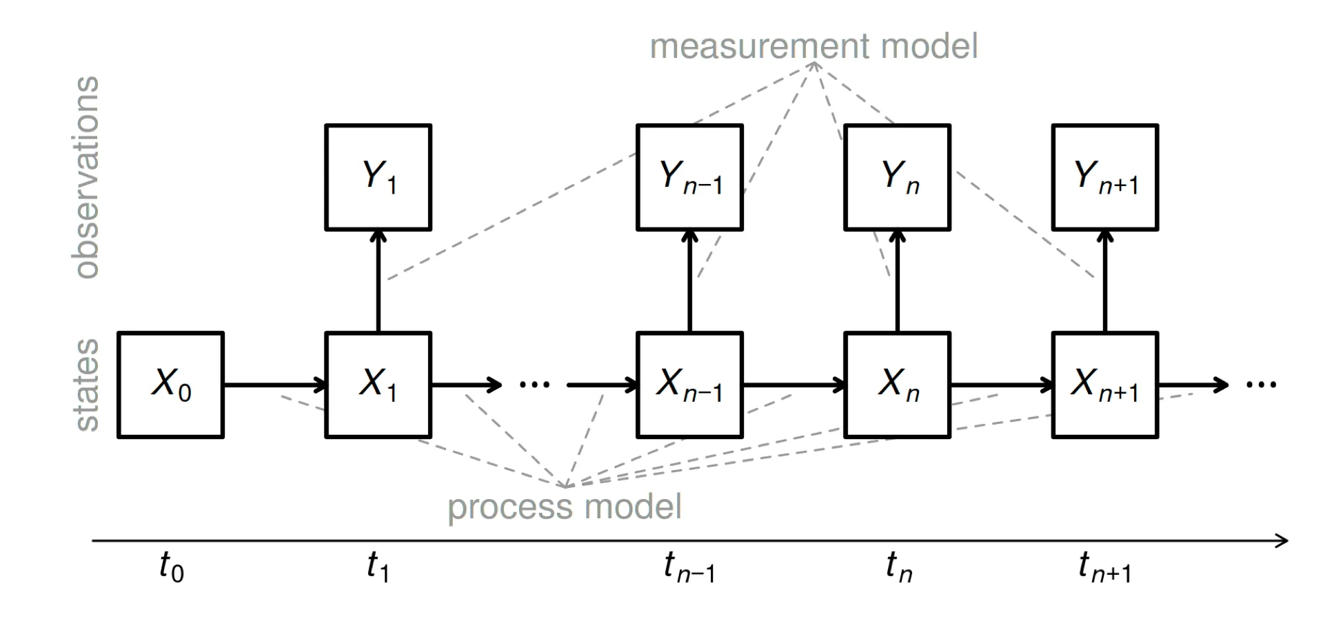
- The state process, $X_n$, is Markovian, i.e., $f_{X_n \vert X_{0:n−1} ,Y_{1:n−1}} (x_n \vert x_{0:n−1} , y_{1:n−1}) = f_{X_n \vert X_{n−1}} (x_n \vert x_{n−1})$.
- Moreover, $Y_n$, depends only on the state at that time: $f_{Y_n \vert X_{0:N},Y_{1:n−1}}(y_n \vert x_{0:n},y_{1:n−1}) = f_{Y_n \vert X_n}(y_n \vert x_n)$, for $n = 1,…,N$.
What is a simulation-based method?
- Simulating random processes is often much easier than evaluating their transition probabilities.
- In other words, we may be able to write rprocess but not dprocess.
- Simulation-based methods require the user to specify rprocess but not dprocess.
- Plug-and-play, likelihood-free and equation-free are alternative terms for “simulation-based” methods.
- Much development of simulation-based statistical methodology has occurred in the past decade.
The pomp package
It is useful to divide the pomp package functionality into different levels:
- Basic model components
rinit: simulator for the initial-state distribution, i.e., the distribution of the latent state at time $t_0$.rprocessanddprocess: simulator and density evaluation procedure, respectively, for the process model.rmeasureanddmeasure: simulator and density evaluation procedure, respectively, for the measurement model.rprioranddprior: simulator and density evaluation procedure, respectively, for the prior distribution.skeleton: evaluation of a deterministic skeleton.partrans: parameter transformations.
-
Workhorses
Workhorses are R functions, built into the package, that cause the basic model component procedures to be executed.
-
Elementary POMP algorithms
These are algorithms that interrogate the model or the model/data confrontation without attempting to estimate parameters. There are currently four of these:
simulateperforms simulations of the POMP model, i.e., it samples from the joint distribution of latent states and observables.pfilterruns a sequential Monte Carlo (particle filter) algorithm to compute the likelihood and (optionally) estimate the prediction and filtering distributions of the latent state process.probecomputes one or more uni or multivariate summary statistics on both actual and simulated data.spectestimates the power spectral density functions for the actual and simulated data.
- Inference algorithms
abc: approximate Bayesian computationbsmc2: Liu-West algorithm for Bayesian SMCpmcmc: a particle MCMC algorithmmif2: iterated filtering (IF2)enkf, eakf ensemble and ensemble adjusted Kalman filterstrajobjfun: trajectory matchingspectobjfun: power spectrum matchingprobeobjfun: probe matchingnlfobjfun: nonlinear forecasting
2: Simulation of stochastic dynamic models
Compartment models
-
A basic SIR model:
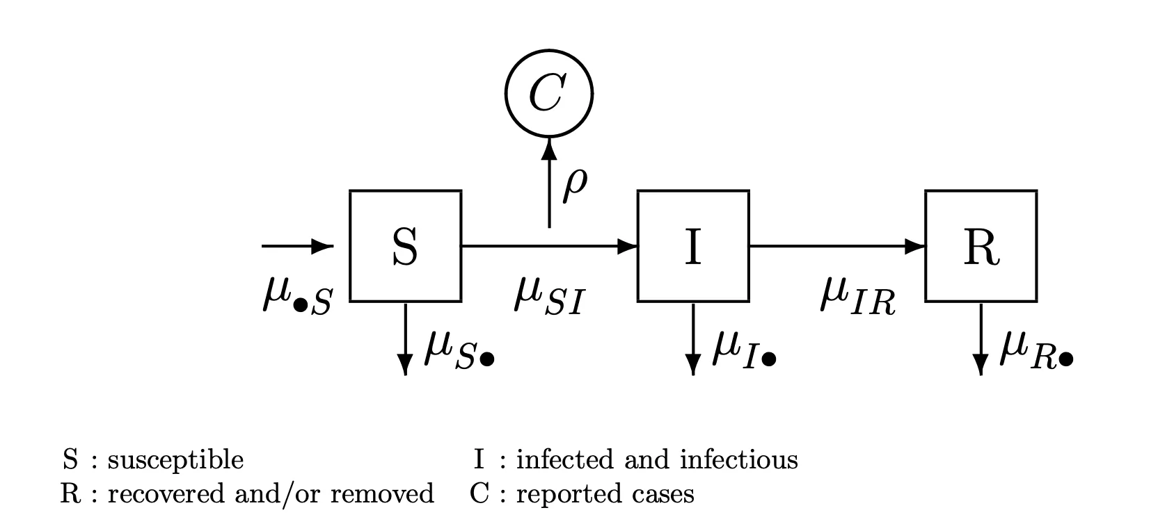
- A deterministic interpretation: \(\frac{dN_{SI}}{dt} = \mu_{SI}(t)S(t)\\ \frac{dN_{IR}}{dt} = \mu_{IR}I(t)\)
- A stochastic interpretation: \(\mathbb{P}(N_{SI}(t+\delta)=N_{SI}(t)+1)=\mu_{SI}(t)S(t)\delta+o(\delta)\\ \mathbb{P}(N_{SI}(t+\delta)=N_{SI}(t))=1-\mu_{SI}(t)S(t)\delta+o(\delta)\\ \mathbb{P}(N_{IR}(t+\delta)=N_{IR}(t)+1)=\mu_{IR}I(t)\delta+o(\delta)\\ \mathbb{P}(N_{IR}(t+\delta)=N_{IR}(t))=1-\mu_{IR}I(t)\delta+o(\delta)\)
Euler’s method
Numerical solution of deterministic dynamics
- Euler’s method for ordinary differential equations Mathematical analysis of Euler’s method says that, as long as the function $h(x)$ is not too exotic, then $x(t)$ is well approximated by $\tilde{x}(t)$ when the discretization time-step, δ, is sufficiently small.
- Numerical solution of stochastic dynamics:
- A Poisson approximation:\(\tilde{N}_{SI}(t+\delta) = \tilde{N}_{SI} + Poisson[\mu_{SI}(\tilde{I}(t))\tilde{S}(t)\delta]\)
- A binomial approximation:\(\tilde{N}_{SI}(t+\delta) = \tilde{N}_{SI} + Binomial[\tilde{S}(t), \mu_{SI}(\tilde{I}(t))\delta]\)
- A binomial approximation with exponential transition probabilities:\(\tilde{N}_{SI}(t+\delta) = \tilde{N}_{SI} + Binomial[\tilde{S}(t), 1-exp\{-\mu_{SI}(\tilde{I}(t))\delta\}]\)
- Analytically, it is usually easiest to reason using (1) or (2). Practically, it is usually preferable to work with (3).
- Numerically, Gillespie’s algorithm is often approximated using so-called tau-leaping methods. These are closely related to Euler’s approach. In this context, the Euler method has sometimes been called tau-leaping.
- For constant-rate compartmental models, the Gillespie algorithm gives an exact solution at the expense of additional computation time. We may on occastion want an exact simulator, and in that case Gillespie can be used.
Compartment models in pomp
- There is a term called accumulator variable in pomp, specified by
accumvars, which will be reset to zero at the beginning of each observation. - C snippets are preferred.
3: Likelihood for POMPs: theory and practice
Introduction
The following schematic diagram represents conceptual links between different components of the methodological approach we’re developing for statistical inference on epidemiological dynamics.
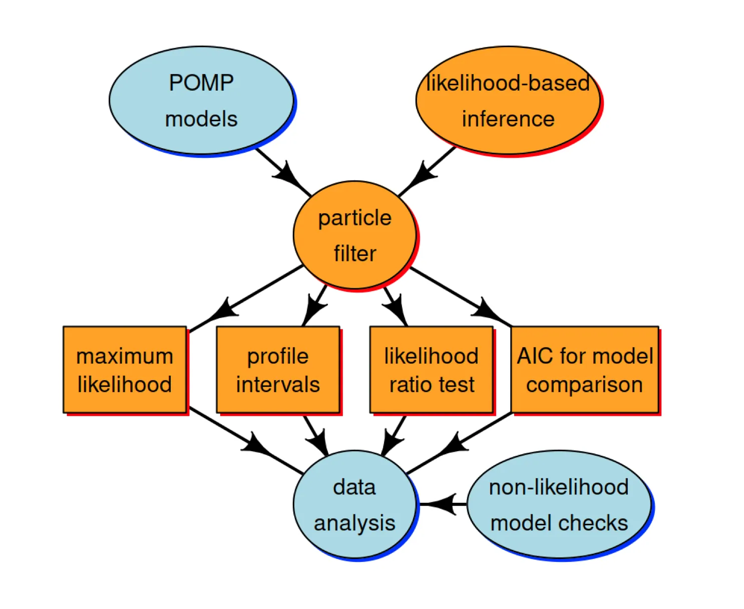
In this lesson, we’re going to discuss the orange compartments. The Monte Carlo technique called the “particle filter” is central for connecting the higher-level ideas of POMP models and likelihood-based inference to the lower-level tasks involved in carrying out data analysis.
The likelihood function
Definition of the likelihood function
\(\mathcal{L}(\theta)=f_{Y_{1:N}}(y_{1:N}^{*};\theta)\) $f_{Y_{1:N}}(y_{1:N};\theta)$ is a probability density function which defines a probability distribution for each value of a parameter vector $\theta$, and $y_{1:N}^{*}$ is the observation, which should be a random draw from the density function.
A simulator is implicitly a statistical model
- For simple statistical models, we may describe the model by explicitly writing the density function $f_{Y_{1:N}}(y_{1:N};\theta)$. One may then ask how to simulate a random variable $Y_{1:N} \sim f_{Y_{1:N}}(y_{1:N};\theta)$.
- For many dynamic models it is much more convenient to define the model via a procedure to simulate the random variable $Y_{1:N}$ . This implicitly defines the corresponding density $f_{Y_{1:N}}(y_{1:N};\theta)$.
Likelihood of a POMP model
- The marginal density for sequence of measurements, $Y_{1:N}$ , evaluated at the data, $y_{1:N}^*$, is \(\begin{align} \mathcal{L}(\theta) &= f_{Y_{1:N}}(y_{1:N}^*;\theta)\\ &= \int{f_{X_{0:N}, Y_{1:N}}(x_{0:N}, y_{1:N}^*;\theta)}dx_{0:N}\\ &= \int{f_{X_0}(x_0;θ) \prod_{n=1}^{N} f_{X_n \vert X_{n−1}}(x_n \vert x_{n−1};θ)f_{Y_n \vert X_n}(y_n^* \vert x_n;θ)}dx_{0:N}, \end{align}\) which can be written as an expectation, \(\mathcal{L}(\theta) = \mathbb{E}[\prod_{n=1}^{N}f_{Y_n \vert X_n}(y_n^* \vert x_n;θ)] ,\) where the expectation is taken with $X_{0:N}$.
- This integral is high dimensional and, except for the simplest cases, can not be reduced analytically.
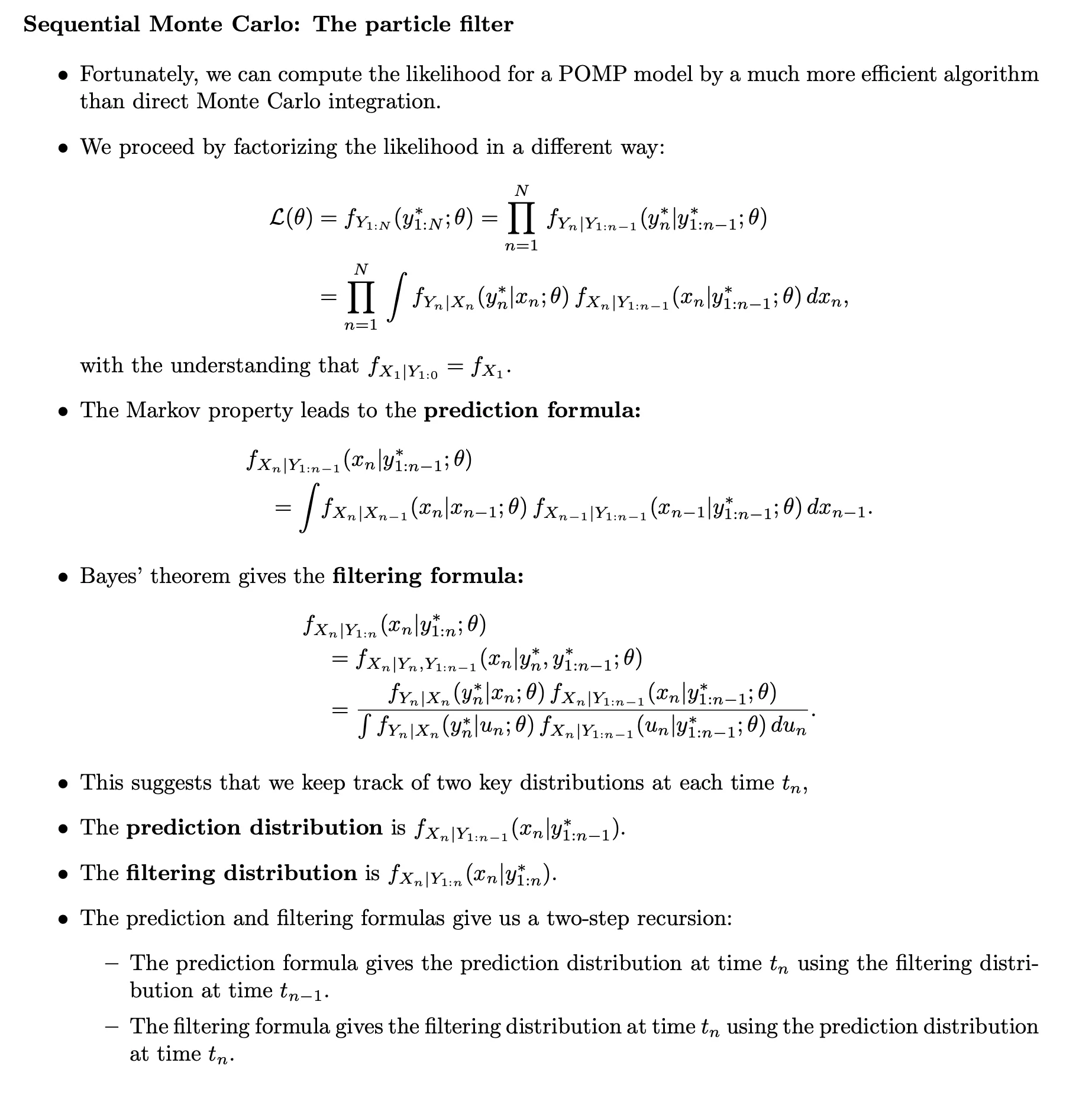
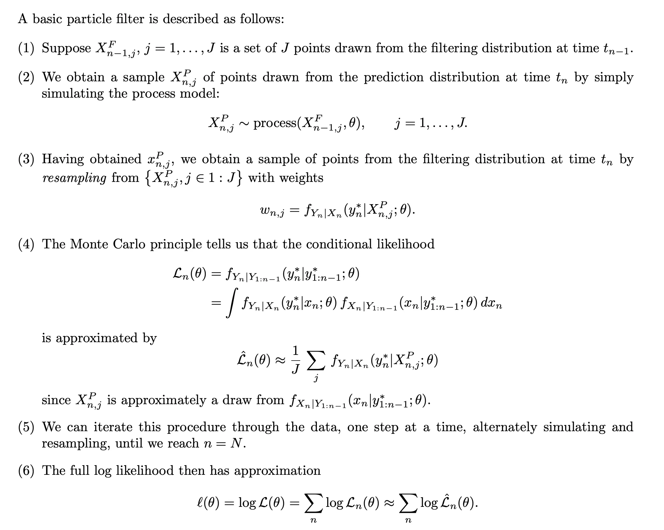
Sequential Monte Carlo: The particle filter
- Particle filter is a much more efficient algorithm than direct Monte Carlo integration.
- Importance sampling can potentially reduce the variance of the Monte Carlo distribution. Illustration please refer to this video.
- A simple video explaining particle filter.
- Essentially, the particle filter weights the prediction particles $X^P_{n,j}$ by the observation data $y^{*}{n}$, then _resample the distribution to obtain a filtering distribution.
- Particle filter in pomp:
foreach (i=1:10, .combine=c) %dopar% {
  library(pomp)
  measSIR %>% pfilter(Np=5000)
} -> pf
logLik(pf) -> ll
logmeanexp(ll,se=TRUE)
                    se
-131.934662    0.684017
Likelihood-based inference
Parameter estimates and uncertainty quantification
There are three main approaches to estimating the statistical uncertainty in an MLE.
- The Fisher information.
- A computationally quick approach when one has access to satisfactory numerical second derivatives of the log likelihood.
- The approximation is satisfactory only when θˆ is well approximated by a normal distribution.
- Neither of the two requirements above are typically met for POMP models.
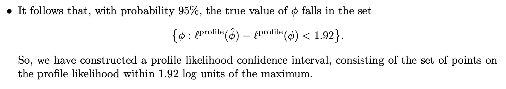
- Profile likelihood estimation. Profile log likelihood function is used in pomp.
- A simulation study, also known as a bootstrap.
- If done carefully and well, this can be the best approach.
- A confidence interval is a claim about reproducibility. You claim, so far as your model is correct, that on 95% of realizations from the model, a 95% confidence interval you have constructed will cover the true value of the parameter.
- A simulation study can check this claim fairly directly, but requires the most effort.
Geometry of the likelihood function
We can use slices to study the log likelihood surface.
More on likelihood-based inference
Maximizing the likelihood
- likelihood maximization might be to stick the particle filter log likelihood estimate into a standard numerical optimizer, such as the Nelder-Mead algorithm. But this approach is unsatisfactory. Standard numerical optimizers are not designed to maximize noisy and computationally expensive Monte Carlo functions.
- We’ll present an iterated filtering algorithm for maximizing the likelihood in a way that takes advantage of the structure of POMP models and the particle filter.
- Likelihood-based model selection and model diagnostics
- For nested hypotheses, we can carry out model selection by likelihood ratio tests.
- For non-nested hypotheses, likelihoods can be compared using Akaike’s information criterion (AIC) or related methods.
Likelihood ratio test
-
Wilks approximation:
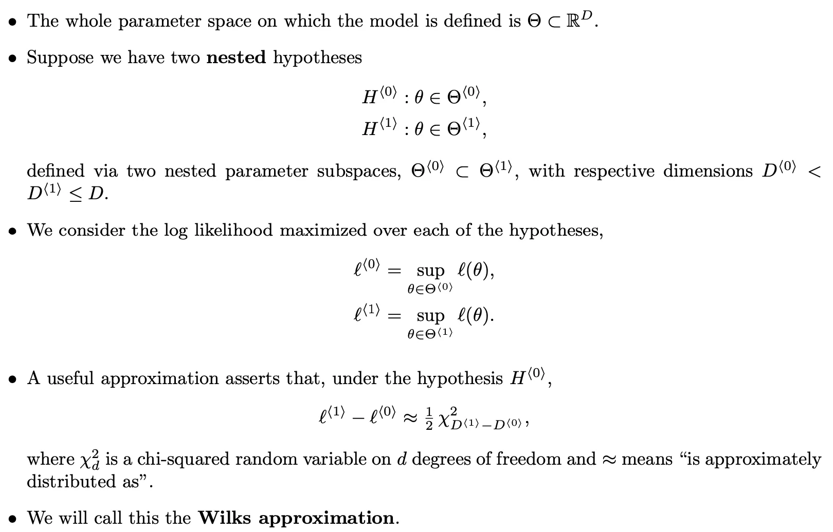
- The Wilks approximation can be used to construct a hypothesis test of the null hypothesis $H^{⟨0⟩}$ against the alternative $H^{⟨1⟩}$.
- This is called a likelihood ratio test since a difference of log likelihoods corresponds to a ratio of likelihoods.
- The chi-squared approximation to the likelihood ratio statistic may be useful, and can be assessed empirically by a simulation study, even in situations that do not formally satisfy any known theorem.
-
Wilks’ theorem and profile likelihood:
Information criteria
- Akaike’s information criterion (AIC) is given by $AIC = −2 \mathbb{l} (\hat{θ}) + 2 D$, “Minus twice the maximized log likelihood plus twice the number of parameters.”
- AIC was derived as an approach to minimizing prediction error. Increasing the number of parameters leads to additional overfitting which can decrease predictive skill of the fitted model.
- AIC does not penalize model complexity beyond the consequence of reduced predictive skill due to overfitting. One can penalize complexity by incorporating a more severe penalty than the 2D term above, such as via BIC.
4: Iterated filtering: principles and practice
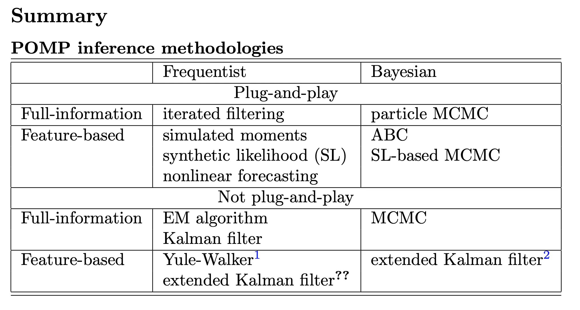
Classification of statistical methods for POMP models
The plug-and-play (Simulation-based) methods
- Inference methodology that calls
rprocessbut notdprocessis said to be plug-and-play. All popular modern Monte Carlo methods fall into this category. - Plug-and-play methods can call
dmeasure. A method that uses only rprocess and rmeasure is called “doubly plug-and-play”. - Two non-plug-and-play methods, expectation-maximization (EM) and Markov chain Monte Carlo (MCMC), have theoretical convergence problems for nonlinear POMP models. The failures of these two workhorses of statistical computation have prompted development of alternative methodologies.
Full information vs. feature-based methods
- Full-information methods are defined to be those based on the likelihood function for the full data (i.e., likelihood-based frequentist inference and Bayesian inference).
- Feature-based methods either consider a summary statistic (a function of the data) or work with an an alternative to the likelihood.
- Asymptotically, full-information methods are statistically efficient and feature-based methods are not.
- In some cases, loss of statistical efficiency might be an acceptable tradeoff for advantages in computational efficiency.
Bayesian vs. frequentist approaches
- Recently, plug-and-play Bayesian methods have been discovered:
- particle Markov chain Monte Carlo (PMCMC) (Andrieu et al., 2010).
- approximate Bayesian computation (ABC) (Toni et al., 2009).
- Prior belief specification is both the strength and weakness of Bayesian methodology:
- The likelihood surface for nonlinear POMP models often contains nonlinear ridges and variations in curvature.
- These situations bring into question the appropriateness of independent priors derived from expert opinion on marginal distributions of parameters.
- They also are problematic for specification of “flat” or “uninformative” prior beliefs.
- Expert opinion can be treated as data for non-Bayesian analysis. However, our primary task is to identify the information in the data under investigation, so it can be helpful to use methods that do not force us to make our conclusions dependent on quantification of prior beliefs.
Summary
Iterated filtering in theory
Full-information, plug-and-play, frequentist methods
- Iterated filtering methods (Ionides et al., 2006, 2015)are the only currently available, full-information, plug-and-play, frequentist methods for POMP models.
- Iterated filtering methods have been shown to solve likelihood-based inference problems for epidemiological situations which are computationally intractable for available Bayesian methodology (Ionides et al., 2015).
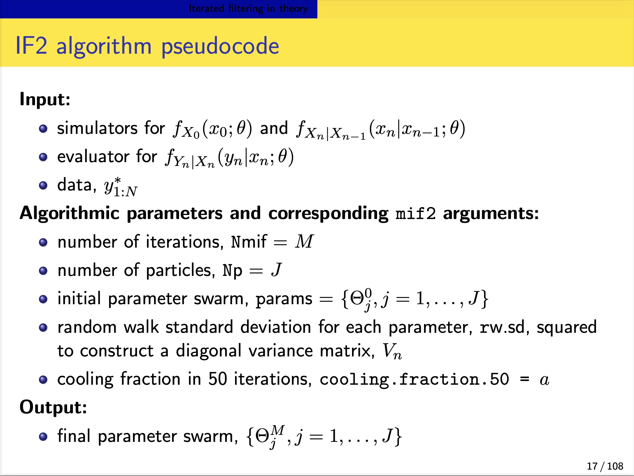
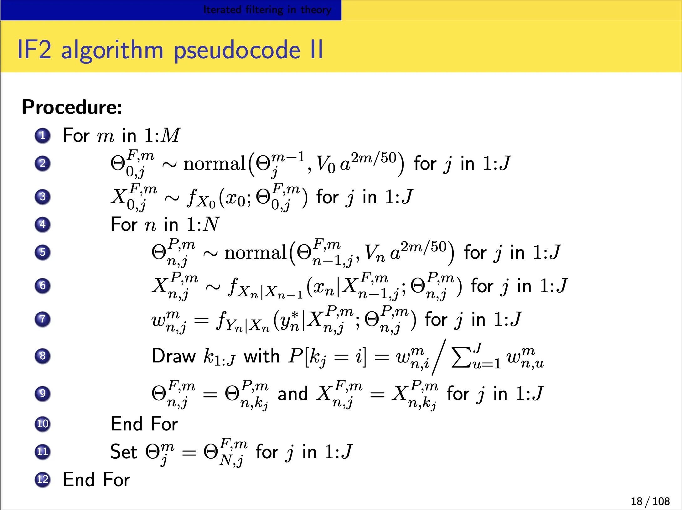
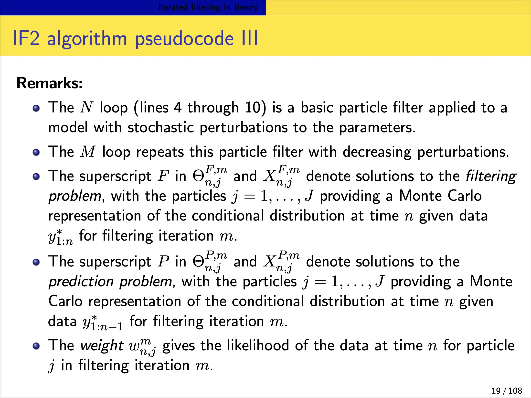
An iterated filtering algorithm (IF2)
We focus on the IF2 algorithm of Ionides et al. (2015). In this algorithm:
- Each iteration consists of a particle filter, carried out with the parameter vector, for each particle, doing a random walk (note the $\Theta^{m}\sim\Theta^{m-1}$ in the below slide).
- At the end of the time series, the collection of parameter vectors is recycled as starting parameters for the next iteration.
-
The random-walk variance decreases at each iteration. In theory, this procedure converges toward the region of parameter space maximizing the maximum likelihood. In practice, we can test this claim on examples.
Iterated filtering in practice
There are many codes in practice in this section. Some key information are listed below.
Local MLE
- we can first explore a point likelihood by particle filter with a initial parameter vector.
- We could then do a local search of the likelihood surface around this point. We will use
mif2in this step to maximize the local likelihood. The likelihood from this step is not good enough for reliable inference, because:- Partly, this is because parameter perturbations are applied in the last filtering iteration, so that the likelihood reported by mif2 is not identical to that of the model of interest.
- Partly, this is because mif2 is usually carried out with fewer particles than are needed for a good likelihood evaluation.
- Therefore, we need to evaluate the likelihood, together with a standard error, using replicated particle filters at each point estimate.
Global MLE
- To perform a global maximum likelihood estimation:
- Practical parameter estimation involves trying many starting values for the parameters.
- One way to approach this is to choose a large box in parameter space that contains all remotely sensible parameter vectors.
- If an estimation method gives stable conclusions with starting values drawn randomly from this box, this gives some confidence that an adequate global search has been carried out.
- We could start with a box of starting parameter vectors, and carry out likelihood maximizations from diverse starting points.
Profile likelihood
- From the global MLE results, we could get a “poor man’s profiles”.
- To perform formal profile likelihood, we’ll first bound the uncertainty by putting a box around the highest-likelihood esti- mates we’ve found so far.
- Within this box, we’ll choose some random starting points, for each of several values of $\eta$, which is the parameter we focuses on.
- Now, we’ll start one independent sequence of iterated filtering operations from each of these points.
- We’ll be careful to keep $\eta$ fixed.
- This is accomplished by not giving this parameter a random perturbation in the
mif2call. - 95%CI of $\eta$ can be obtained through this procedure.
- As one varies $\eta$ across the profile, the model compensates by adjusting the other parameters.
- It can be very instructive to understand how the model does this.
- For example, how does the reporting efficiency, $\rho$, change as $\eta$ is varied?
- We can plot ρ vs $\eta$ across the profile.
- This is called a profile trace.
The investigation continues
- If we found that some of the parameter estimation is in conflict of some existing knowledge, we may need to adjust the model, e.g. relax some parameters and fixed some others.
- In iterated filtering, We could adopt a simulated tempering approach (following a metallurgical analogy), in which we increase the size of the random perturbations some amount (i.e., “reheat”), and then continue cooling.
mf %>% mif2(
    Nmif=100,rw.sd=rw.sd(Beta=0.01,mu_IR=0.01,eta=ivp(0.01))
  ) %>%
  mif2(
    Nmif=100,
    rw.sd=rw.sd(Beta=0.005,mu_IR=0.005,eta=ivp(0.005))
) -> mf
5. Case study: measles. Recurrent epidemics, long time series, covariates, extra-demographic stochasticity, interpretation of parameter estimates.
Objectives
- To display a published case study using plug-and-play methods with non-trivial model complexities.
- To show how extra-demographic stochasticity can be modeled.
- To demonstrate the use of covariates in pomp.
- To demonstrate the use of profile likelihood in scientific inference.
- To discuss the interpretation of parameter estimates.
- To emphasize the potential need for extra sources of stochasticity in modeling.
Model and implementation
Data sets
Measles in England and Wales
- He, Ionides, & King, J. R. Soc. Interface (2010)
- Twenty towns, including
- 10 largest
- 10 smaller, chosen at random
- Population sizes: 2k–3.4M
- Weekly case reports, 1950–1963
- Annual birth records and population sizes, 1944–1963
Modeling
Continuous-time Markov process model:
- Covariates: Birth rates and population size
- Entry into susceptible class: Considered cohort effect and school entry delay.
- Force of infection: considered imported infections, gamma white noise, and seasonality if school term.
- Overdispersed binomial measurement model
Model implementation in pomp, estimation and simulation
R script is available.
Basically, we define rprocess, rmeasure and dmaeasure in Csnippet, then put in the pomp object, then run global mle estimation and then inference from mle.
The fitting procedure used is as follows:
- A large number of searches were started at points across the parameter space.
- Iterated filtering was used to maximize the likelihood.
- We obtained point estimates of all parameters for 20 cities.
- We constructed profile likelihoods to quantify uncertainty in London and Hastings.
Note that we should also use parameter transformations when doing likelihood maximization. Specifically, to enforce positivity, we log transform, to constrain parameters to (0,1), we logit transform, and to confine parameters to the unit simplex, we use the log-barycentric transformation.
6: Case study: Polio
Objectives
- Demonstrate the use of covariates in pomp to add demographic data (birth rates and total population) and seasonality to an epidemiological model.
- Show how partially observed Markov process (POMP) models and methods can be used to understand transmission dynamics of polio.
- Practice maximizing the likelihood for such models. How to set up a global search for a maximum likelihood estimate. How to assess whether a search has been successful.
- Provide a workflow that can be adapted to related data analysis tasks.
Covariates
- Suppose our time series of primary interest is $y_{1:N}$.
- A covariate time series is an additional time series $z_{1:N}$ which is used to help explain $y_{1:N}$.
- When the process leading to $z_{1:N}$ is not external to the system generating it, we must be alert to the possibility of reverse causation and confounding variables.
A POMP model for polio
The process model is illustrated as below:
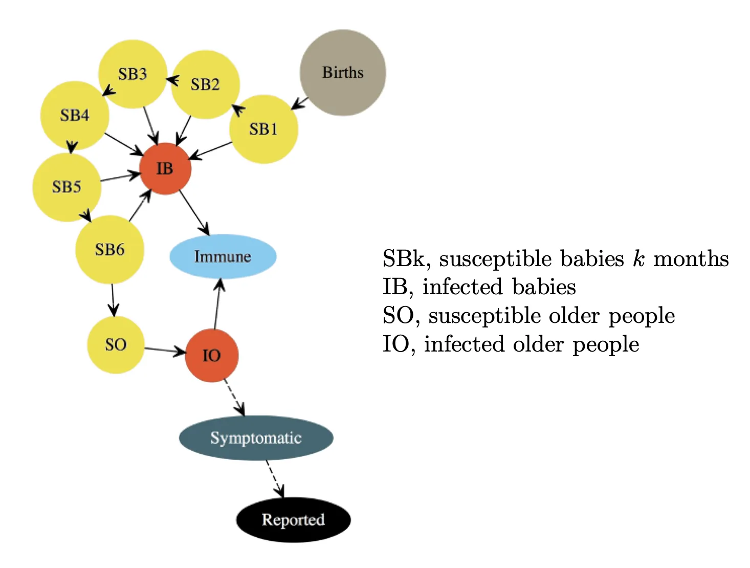
The measurement model is a discretized normal distribution truncated at zero, with both environmental and Poisson-scale contributions to the variance: \(\begin{align*} Y_n=max\{round(Z_n, 0)\}, \\ Z_n \sim normal(\rho I^{O}_{n}, (\tau I^{O}_{n})^2+\rho I^{O}_{n}). \end{align*}\)
A pomp representation of the POMP model
Details please see the R scripts, the scripts for this section is very helpful.
Logistics for the computations
Controlling run time
Setting run levels to control computation time
run_level=1will set all the algorithmic parameters to the first column of values in the following code, for debugging.- Here, Np is the number of particles, Nmif is the number of iterations of the optimization procedure carried, other variables are defined for use later.
run_level=2uses enough effort to gives reasonably stable results at a moderate computational time.- Larger values give more refined computations, implemented here by
run_level=3which was run on a computing cluster.run_level <- 3 Np <- switch(run_level,100, 1e3, 5e3) Nmif <- switch(run_level, 10, 100, 200) Nreps_eval <- switch(run_level, 2, 10, 20) Nreps_local <- switch(run_level, 10, 20, 40) Nreps_global <-switch(run_level, 10, 20, 100) Nsim <- switch(run_level, 50, 100, 500)
Setting up parallelization
We will use doFuture to parallelize our computations. At run-levels 1 and 2, it will be sufficient to use the multiple cores on a single machine, but at run-level 3, we will use an HPC cluster. In the following, we use our own HPC cluster. To run these codes on your own HPC cluster, you would need to edit the CLUSTER.R script suitably.
library(doFuture)
library(iterators)
par_init <- function (run_level) {
if (run_level >= 3 && file.exists("CLUSTER.R")) {
source("CLUSTER.R") } else {
plan(multisession) }
}
Parallel computation of the likelihood
Likelihood evaluation at the starting parameter estimate
stew(file="pf1.rda",seed=3899882,{
  par_init(run_level)
  pf1 <- foreach(i=1:20,.combine=c,
    .options.future=list(seed=TRUE)
  ) %dofuture% pfilter(polio,Np=Np)
  cores <- nbrOfWorkers()
})
L1 <- logmeanexp(sapply(pf1,logLik),se=TRUE)
Simulation
Simulation to investigate local persistence
For Wisconsin, using our model at the estimated MLE, we simulate in parallel as follows:
simulate(polio,nsim=Nsim,seed=1643079359,
  format="data.frame",include.data=TRUE) -> sims
Likelihood maximization
Local likelihood maximization
Let’s see if we can improve on the previous MLE (starting parameter estimate). We use the IF2 algorithm. We set a constant random walk standard deviation for each of the regular parameters and a larger constant for each of the initial value parameters:
mif.rw.sd <- eval(substitute(rw_sd(
  b1=rwr,b2=rwr,b3=rwr,b4=rwr,b5=rwr,b6=rwr,
  psi=rwr,rho=rwr,tau=rwr,sigma_dem=rwr,
  sigma_env=rwr,
  IO_0=ivp(rwi),SO_0=ivp(rwi)),
  list(rwi=0.2,rwr=0.02)))

stew(file="mif.rda",seed=942098028,{
  par_init(run_level)
  m2 <- foreach(
    i=1:Nreps_local,.combine=c,
    .options.future=list(seed=TRUE)
  ) %dofuture%
    mif2(polio, Np=Np, Nmif=Nmif, rw.sd=mif.rw.sd,
      cooling.fraction.50=0.5)
  lik_m2 <- foreach(
    m=m2,.combine=rbind,
    .options.future=list(seed=TRUE)
  ) %dofuture%
    logmeanexp(replicate(Nreps_eval,
logLik(pfilter(m,Np=Np))),se=TRUE)
})

coef(m2) |> melt() |> spread(name,value) |>
  select(-.id) |>
  bind_cols(logLik=lik_m2[,1],logLik_se=lik_m2[,2]) -> r2
r2 |> arrange(-logLik) |>
  write_csv("params.csv")
Global likelihood maximization
- Practical parameter estimation involves trying many starting values for the parameters. One can specify a large box in parameter space that contains all sensible parameter vectors.
- If the estimation gives stable conclusions with starting values drawn randomly from this box, we have some confidence that our global search is reliable.
- For our polio model, a reasonable box might be:
box <- rbind(
  b1=c(-2,8), b2=c(-2,8),
  b3=c(-2,8), b4=c(-2,8),
  b5=c(-2,8), b6=c(-2,8),
  psi=c(0,0.1), rho=c(0,0.1), tau=c(0,0.1),
  sigma_dem=c(0,0.5), sigma_env=c(0,1),
  SO_0=c(0,1), IO_0=c(0,0.01)
)

bake(file="box_eval1.rds",seed=833102018,{
  par_init(run_level)
  foreach(i=1:Nreps_global,.combine=c,
    .options.future=list(seed=TRUE)) %dofuture%
    mif2(m2[[1]],params=c(fixed_params,
      apply(box,1,function(x)runif(1,x[1],x[2]))))
}) -> m3

bake(file="box_eval2.rds",seed=71449038,{
  par_init(run_level)
  foreach(m=m3,.combine=rbind,
    .options.future=list(seed=TRUE)) %dofuture%
    logmeanexp(replicate(Nreps_eval,
      logLik(pfilter(m,Np=Np))),se=TRUE)
}) -> lik_m3

coef(m3) |> melt() |> spread(name,value) |>
  select(-.id) |>
  bind_cols(logLik=lik_m3[,1],logLik_se=lik_m3[,2]) -> r3
read_csv("params.csv") |>
  bind_rows(r3) |>
  arrange(-logLik) |>
  write_csv("params.csv")
summary(r3$logLik,digits=5)
Benchmark likelihoods for non-mechanistic models
- To understand these global searches, many of which may correspond to parameter values having no meaningful scientific interpretation, it is helpful to put the log-likelihoods in the context of some non-mechanistic benchmarks.
- The most basic statistical model for data is independent, identically distributed (IID). Picking a negative binomial model,
nb_lik <- function (theta) {
  -sum(dnbinom(as.numeric(obs(polio)),size=exp(theta[1]),prob=exp(theta[2]),log=TRUE))}
nb_mle <- optim(c(0,-5),nb_lik)
-nb_mle$value

[1] -1036.227
ARMA models as benchmarks
log_y <- log(as.vector(obs(polio))+1)
arma_fit <- arima(log_y,order=c(2,0,2),
  seasonal=list(order=c(1,0,1),period=12))
arma_fit$loglik-sum(log_y)
[1] -822.0827
Profile likelihood
- From the global MLE results, we could get a “poor man’s profiles”.
- To perform formal profile likelihood, we’ll first bound the uncertainty by putting a box around the highest-likelihood estimates we’ve found so far.
library(tidyverse)
params |>
  filter(logLik>max(logLik)-20) |>
  select(-logLik,-logLik_se) |>
  gather(variable,value) |>
  group_by(variable) |>
  summarize(min=min(value),max=max(value)) |>
  ungroup() |>
  column_to_rownames(var="variable") |>
  t() -> box

profile_pts <-  switch(run_level,  3,  5,  30)
profile_Nreps <- switch(run_level, 2,  3,  10)

idx <- which(colnames(box)!="rho")
profile_design(
  rho=seq(0.01,0.025,length=profile_pts),
  lower=box["min",idx],upper=box["max",idx],
  nprof=profile_Nreps
) -> starts

profile.rw.sd <- eval(substitute(rw_sd(
  rho=0,b1=rwr,b2=rwr,b3=rwr,b4=rwr,b5=rwr,b6=rwr,
  psi=rwr,tau=rwr,sigma_dem=rwr,sigma_env=rwr,
  IO_0=ivp(rwi),SO_0=ivp(rwi)),
  list(rwi=0.2,rwr=0.02)))

stew(file="profile_rho.rda",seed=1888257101,{
  par_init(run_level)

  foreach(start=iter(starts,"row"),.combine=rbind,
.options.future=list(seed=TRUE)) %dofuture% {

    polio |> mif2(params=start,
      Np=Np,Nmif=ceiling(Nmif/2),
      cooling.fraction.50=0.5,
      rw.sd=profile.rw.sd
    ) |>
      mif2(Np=Np,Nmif=ceiling(Nmif/2),
        cooling.fraction.50=0.1
      ) -> mf

    replicate(Nreps_eval,
      mf |> pfilter(Np=Np) |> logLik()
    ) |> logmeanexp(se=TRUE) -> ll

    mf |> coef() |> bind_rows() |>
      bind_cols(logLik=ll[1],logLik_se=ll[2])
  } -> m4

  cores <- nbrOfWorkers()
})
Exercise 6.5. Diagnosing filtering and maximization convergence
https://kingaa.github.io/sbied/polio/convergence-exercise.html
7: Case study: forecasting Ebola
Introduction
Objectives
- To explore the use of POMP models in the context of an outbreak of an emerging infectious disease.
- To demonstrate the use of diagnostic probes for model criticism.
- To illustrate some forecasting methods based on POMP models.
- To provide an example that can be modified to apply similar approaches to other outbreaks of emerging infectious diseases.
Best practices
The paper recommended the use of POMP models, for several reasons:
- Such models can accommodate a wide range of hypothetical forms.
- They can be readily fit to incidence data, especially during the exponential growth phase of an outbreak.
- Stochastic models afford a more explicit treatment of uncertainty.
- POMP models come with a number of diagnostic approaches built-in, which can be used to assess model misspecification
Data and model
SEIR model with gamma-distributed latent period
Specifically, this model assumes that the amount of time an infection remains latent is \(LP \sim Gamma(m, \frac{1}{m\alpha}),\) where $m$ is a integer. This means that the latent period has expectation $\frac{1}{\alpha}$ and variance $\frac{1}{m\alpha}$. In this document, where $m$ is an integer. we’ll fix $m = 3$. We implement Gamma distributions using the so-called linear chain trick (divide the E compartment into $m$ linked sub-compartments).
The observations are modeled as a negative binomial process conditional on the number of infections. The negative binomial process allows for overdispersion in the counts. This overdispersion is controlled by parameter $k$.
Model criticism
The guiding principle in this is that, if the model is “good”, then the data are a plausible realization of that model. Therefore, we can compare the data directly against model simulations. Moreover, we can quantify the agreement between simulations and data in any way we like. Shortcomings of the model should manifest themselves as discrepancies between the model-predicted distribution of such statistics and their value on the data. Specifically, the probe function applies a set of user-specified summary statistics or probes, to the
model and the data, and quantifies the degree of disagreement in several ways.
Simulation for diagnosis
profs |>
  filter(country=="Guinea") |>
  filter(loglik==max(loglik)) |>
  select(-loglik,-loglik.se,-country,-profile) -> coef(gin)

gin |>
  simulate(nsim=20,format="data.frame",include.data=TRUE) |>
  mutate(
    date=min(dat$date)+7*(week-1),
    is.data=ifelse(.id=="data","yes","no")
  ) |>
  ggplot(aes(x=date,y=cases,group=.id,color=is.data,alpha=is.data))+
  geom_line()+
  guides(color="none",alpha="none")+
  scale_color_manual(values=c(no=gray(0.6),yes="red"))+
  scale_alpha_manual(values=c(no=0.5,yes=1))
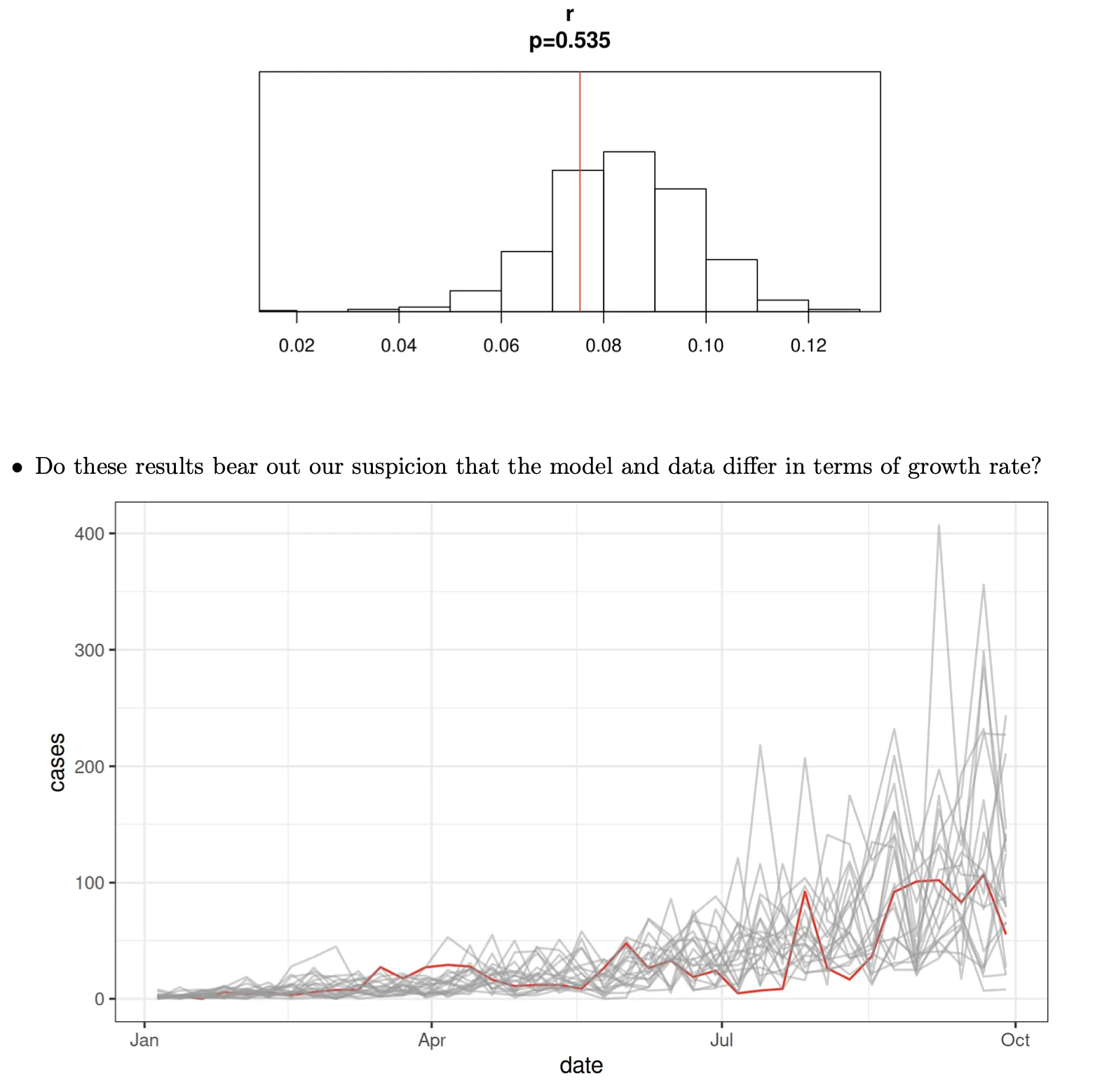
Diagnostic probes
- Does the data look like it could have come from the model?
- The simulations appear to be growing a bit more quickly than the data.
- Let’s try to quantify this.
- First, we’ll write a function that estimates the exponential growth rate by linear regression.
- Then, we’ll apply it to the data and to 500 simulations.
- In the following, gin is a pomp object containing the model and the data from the Guinea outbreak.
growth.rate <- function (y) {
  cases <- y["cases",]
  fit <- lm(log1p(cases)~seq_along(cases))
  unname(coef(fit)[2])
}

gin |>
  probe(probes=list(r=growth.rate),nsim=500) |>
  plot()
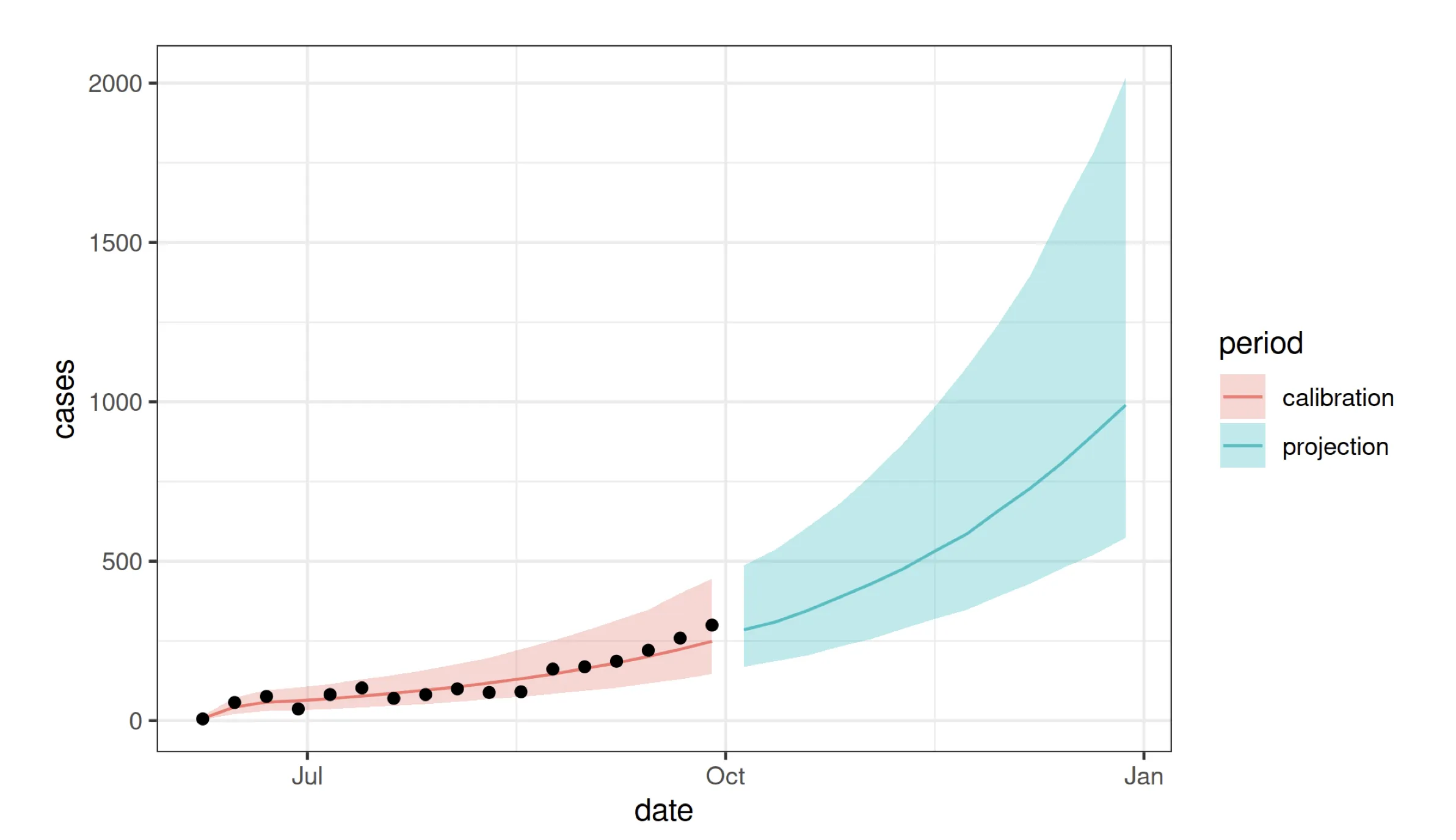
Forcasting using POMP models
Sources of uncertainty
A set of key issues surrounds quantifying the forecast uncertainty. This arises from four sources:
- measurement error
- process noise
- parametric uncertainty
- structural uncertainty Here, we’ll explore how we can account for the first three of these in making forecasts for the Sierra Leone outbreak.
Forecasting Ebola: an empirical Bayes approach
Parameter uncertainty
We take an empirical Bayes approach. First, we set up a collection of parameter vectors in a neighborhood of the maximum likelihood estimate containing the region of high likelihood.
profs |>
  filter(country=="SierraLeone") |>
  select(-country,-profile,-loglik.se) |>
  filter(loglik>max(loglik)-0.5*qchisq(df=1,p=0.99)) |>
  gather(parameter,value) |>
  group_by(parameter) |>
  summarize(min=min(value),max=max(value)) |>
  ungroup() |>
  filter(parameter!="loglik") |>
  column_to_rownames("parameter") |>
  as.matrix() -> ranges

sobol_design(
  lower=ranges[,"min"],
  upper=ranges[,"max"],
  nseq=20
) -> params
Process noise and measurement error
Next, we carry out a particle filter at each parameter vector, which gives us estimates of both the likelihood and the filter distribution at that parameter value.
## ----forecasts2a----------------------------------------------------------
bake(file="forecasts.rds",{
  library(doFuture)
  library(iterators)
  plan(multisession)

## ----forecasts2b----------------------------------------------------------
# We repeat this procedure for each parameter vector, binding the results into a single data frame.
  foreach(p=iter(params,by="row"),
    .combine=bind_rows,
    .options.future=list(seed=887851050L)
  ) %dopar% {

## ----forecasts2c----------------------------------------------------------
    M1 <- ebolaModel("SierraLeone")
    M1 |> pfilter(params=p,Np=2000,save.states=TRUE) -> pf

## ----forecasts2d----------------------------------------------------------
# We extract the state variables at the end of the data for use as initial conditions for the forecasts.
    pf |>
      saved_states() |> ## latent state for each particle
      tail(1) |>        ## last timepoint only
      melt() |>         ## reshape and rename the state variables
      pivot_wider() |>
      group_by(.id) |>
      summarize(S_0=S, E_0=E1+E2+E3, I_0=I, R_0=R) |>
      pivot_longer(-.id) |>
      spread(.id,value) |>
      column_to_rownames("name") |>
      as.matrix() -> x
# The final states are now stored in x.

## ----forecasts2e1----------------------------------------------------------
# We simulate forward from the initial condition, up to the desired forecast horizon, to give a forecast corresponding to the selected parameter vector. To do this, we first set up a matrix of parameters:
    pp <- parmat(unlist(p),ncol(x))

## ----forecasts2e2----------------------------------------------------------
# Then, we generate simulations over the “calibration period” (i.e., the time interval over which we have data). We record the likelihood of the data given the parameter vector:
    M1 |>
      simulate(params=pp,format="data.frame") |>
      select(.id,week,cases) |>
      mutate(
        period="calibration",
        loglik=logLik(pf)
      ) -> calib

## ----forecasts2f----------------------------------------------------------
# Now, we create a new pomp object for the forecasting.
    M2 <- M1
    time(M2) <- max(time(M1))+seq_len(horizon)
    timezero(M2) <- max(time(M1))

## ----forecasts2g----------------------------------------------------------
# We set the initial conditions to the ones determined above and perform forecast simulations.
    pp[rownames(x),] <- x

    M2 |>
      simulate(params=pp,format="data.frame") |>
      select(.id,week,cases) |>
      mutate(
        period="projection",
        loglik=logLik(pf)
      ) -> proj

## ----forecasts2h----------------------------------------------------------
# We combine the calibration and projection simulations into a single data frame.
    bind_rows(calib,proj) -> sims

  }
}) -> sims

## ----forecasts2j----------------------------------------------------------
# We give these prediction distributions weights proportional to the estimated likelihoods of the parameter vectors.
sims |>
  mutate(weight=exp(loglik-mean(loglik))) |>
  arrange(week,.id) -> sims

## ----forecasts2k----------------------------------------------------------
# We verify that our effective sample size is large.
sims |>
  filter(week==max(week)) |>
  summarize(ess=sum(weight)^2/sum(weight^2))
# ess: 10485.34

## ----forecasts2l----------------------------------------------------------
# Finally, we compute quantiles of the forecast incidence.
sims |>
  group_by(week,period) |>
  reframe(
    p=c(0.025,0.5,0.975),
    value=wquant(cases,weights=weight,probs=p),
    name=c("lower","median","upper")
  ) |>
  select(-p) |>
  pivot_wider() |>
  ungroup() |>
  mutate(date=min(dat$date)+7*(week-1)) -> simq

## ----forecast-plots,echo=FALSE-------------------------------------------
simq |>
  ggplot(aes(x=date))+
  geom_ribbon(aes(ymin=lower,ymax=upper,fill=period),alpha=0.3,color=NA)+
  geom_line(aes(y=median,color=period))+
  geom_point(data=filter(dat,country=="SierraLeone"),
    mapping=aes(x=date,y=cases),color="black")+
  labs(y="cases")
8: Case study: Sexual contacts panel data
Objectives
- Discuss the use of partially observed Markov process (POMP) methods for panel data, also known as longitudinal data.
- See how POMP methods can be used to understand the outcomes of a longitudinal behavioral survey on sexual contact rates.
- Introduce the R package
panelPompthat extends pomp to panel data.
I am not going to go into details on this section.
Tags: Infectious disease modelling
Categories: Course notes
Comments