Paper digest: Efficient Bayesian inference under the structured coalescent (Timothy G. Vaughan et al., 2014)

This is the paper for MultiTypeTree.

In this article, we present a new MCMC sampler capable of sampling from posterior distributions over structured trees: timed phylogenetic trees in which lineages are associated with the distinct subpopulation in which they lie. The sampler includes a set of MCMC proposal functions that offer significant mixing improvements over a previously published method.

Vaughan, T. G., et al. (2014). Efficient Bayesian inference under the structured coalescent. Bioinformatics. Link

Introduction

• Two MCMC schemes have been proposed for the structured coalescent:
  • The first is the method developed by Beerli and Felsenstein (Beerli, 2006; Beerli and Felsenstein, 1999, 2001), implemented in the software package Migrate-n. This approach uses a single proposal function that updates the structured tree by dissolving a randomly selected edge and drawing a new edge through simulation from the structured coalescent, conditioned on the remaining edges.
  • The second scheme, proposed by Ewing et al. (2004), employs a set of simple and efficient proposal functions focused exclusively on migration events within the structured genealogy. Combined with methods for exploring the space of unstructured trees (Drummond et al., 2002), Ewing et al. demonstrated that this MCMC algorithm can not only jointly infer structured trees and migration parameters but also leverage serially sampled data to estimate absolute migration rates.
• These two methods are slow. In this article, the authors present a new set of MCMC proposal functions (or ‘operators’) designed to efficiently utilize serially sampled sequence data for inferring the complete structured tree and associated model parameters, including mutation rates, within the structured coalescent framework.

Mathematical Background

Definitions

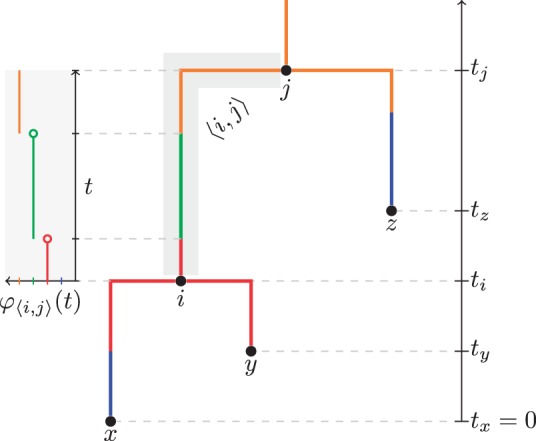
• A structured tree $\mathcal{T}$ of n leaves is a fully resolved, rooted and timed phylogenetic tree. $\mathcal{T}=(V, E, \mathbf{t}, M)$. $V$ is the set of nodes, $E$ is the set of edges, $\mathbf{t}$ is the vector of node times, and $M$ is the set of migration events. The demes are represented by a set $D$.
• The final element in $\mathcal{T}$ is the one that is unique to structured trees and is defined by $M = \lbrace\varphi_{\langle i,j \rangle} \mid \langle i,j \rangle \in E\rbrace$, where each function $\varphi_{\langle i,j \rangle} : [t_i, t_j] \to D$ is piecewise constant and defined such that $\varphi_{\langle i,j \rangle}(t)$ is the type associated with the time $t$ on edge $\langle i,j \rangle \in E$. Such a tree is illustrated in Figure 1.
  • 

Bayseian inference framework

• Sampled individuals are represented by the set $I$, the aligned sequences by the set $S = \lbrace s_i \vert i \in I\rbrace$, the sampling dates by the set $\mathbf{t}_I = \lbrace\mathbf{t}_i \vert i \in I\rbrace$, $\mathbf{t}_Y$ is the vector of internal node times, and the sampling locations by the set $L = \lbrace l_i \vert i \in I\rbrace$. In addition to the parameters of primary interest, $m$ and $\theta$, $\mu$ the nucleotide substitution rate matrix, and $M$ the migration history of lineages in the tree, i.e., the timing, source, sink, and lineage involved in each migration event.

  • Formally, the target of inference is the posterior distribution of the parameters given the data:

    \[P(E, \mathbf{t}_Y, M, \mu, m, \theta \mid S, \mathbf{t}_I, L) \propto P_F(S \mid E, \mathbf{t}, \mu) P(E, \mathbf{t}_Y, M \mid \mathbf{t}_I, L, m, \theta) P(\mu, m, \theta).\]

  • The first term is the phylogenetic tree likelihood, the second term is the structured coalescent likelihood, and the third term is the prior distribution of the parameters.

The structured coalescent probability density

• The probability density of a structured tree:

  \[P(E, t_Y, M \mid t_I, L, m, \theta) = \exp \left[ -\sum_{\alpha=1}^B \tau_\alpha \sum_{d \in D} \left( \binom{k_{\alpha,d}}{2} \frac{1}{\theta_d} + k_{\alpha,d} \sum_{d' \in D \setminus \lbrace d \rbrace} m_{dd'} \right) \right] \times (m_{dd'})^{v^m_{dd'}} \left(\frac{1}{\theta_d}\right)^{v^c_d}.\]
  • The exponential term is the probability of waiting time for the first event to happen
  • Times the probability of the actual events (migrations/coalescences) that do occur.
• Heterochronous (Serial) Sampling
  • The model allows leaf nodes (samples) at different times, which are “sampling events.”
  • The formula extends standard structured coalescent approaches to handle tips sampled at multiple points in time (rather than all at the present).

• There is another formulation from New Routes to Phylogeography: A Bayesian Structured Coalescent Approximation by Nicola De Maio et al. on PLOS Genetics, 2015, which I think is more intuitive.

  1. Basic Idea
     In the structured coalescent, lineages can:
     • Coalesce within the same deme (subpopulation).
     • Migrate from one deme to another.
     • Be sampled at known times (for heterochronous datasets).

     We divide the entire time span (from root to present) into consecutive intervals $\tau_i$.
     Each interval ends when an event actually occurs (coalescence, migration, or sampling).

  2. Two Components per Interval
     For each interval $i$ of length $\tau_i$, the probability contribution $L_i$ has:
     1. An exponential term for waiting time during $\tau_i$.
     2. A multiplier $E_i$ for “which event occurs” at the end of $\tau_i$.

     Thus: \(L_i \;=\; \exp\!\Bigl[ -\,\tau_i \sum_{d\in D} \Bigl( \binom{k_{i,d}}{2} \,\tfrac{1}{\theta_d} \;+\; k_{i,d} \sum_{d'\neq d} m_{dd'} \Bigr) \Bigr] \;\times\; E_i,\) where:

     • $k_{i,d}$ is the number of lineages in deme $d$ during interval $i$.
     • $\theta_d$ is the scaled population size for deme $d$.
     • $m_{dd’}$ is the rate of migration from deme $d’$ to $d$.
  3. Interpreting the Exponential Term
     • $\exp[-(\text{total rate}) \times \tau_i]$ is the probability that no coalescence or migration events happen before $\tau_i$.
     • The total rate is the sum of coalescent rates ($\binom{k_{i,d}}{2}\,\frac{1}{\theta_d}$) and migration rates ($k_{i,d}\,\sum_{d’\neq d} m_{dd’}$) across all demes $d$.
  4. Event Probability Factor $(E_i)$
     After waiting $\tau_i$ with no events, one event happens at the end of interval $i$.
     • Coalescence in deme $d$ adds a factor $\tfrac{1}{\theta_d}$.
     • Migration from $d’$ to $d$ adds a factor $m_{dd’}$.
     • Sampling contributes a factor of 1 (it does not arise from a “rate” in the same sense, but rather is determined by the sampling design).
  5. Multiplying Over All Intervals
     We typically write the full likelihood for the entire genealogy as the product of the $L_i$ factors across intervals $i = 1, 2, \dots, B$: \(P(\text{structured tree}) \;=\; \prod_{i=1}^B L_i.\) This product describes both:
     1. The waiting times (no events) in each interval.
     2. The specific type of event that ends each interval.
  6. Why It Works
     • Poisson Process Logic: Coalescent and migration follow Poisson processes. The probability of no event over $\tau_i$ is an exponential.
     • Single Event at Interval End: We account for the single event by multiplying the appropriate rate parameter (or 1 for sampling).
     • Structured Constraint: Coalescence only occurs when lineages share the same deme. Migration changes deme assignment. Sampling is taken as known.

MCMC Sampling Algorithm

• Structured Tree Operators: Operators adapted from Drummond et al. (2002) include:
  • Wilson-Balding Move: Adjusts subtree attachment.
  • Subtree Exchange Move: Switches subtree connections.
  • Node Height Shifting Move: Adjusts internal node heights.
  • Tree Height Scaling Move: Scales overall tree height.

Implementation and application

• The authors then validate the performance of the model using simulated data.

  • Inference from Simulated Data: The implemented MCMC sampler was tested using simulated data to validate its ability to recover evolutionary and demographic parameters accurately under known conditions.

  • Data Simulation Procedure:
    1. A structured coalescent model was defined with specific types ($D$), immigration rate matrix ($m$), and population size vector ($\theta$).
    2. A 128-taxon structured coalescent tree was simulated using the MASTER tool, with leaf node times spread across $t = 0, 1, 2, 3$, and leaf types distributed evenly across $D$.
    3. A 2 kb nucleotide sequence was evolved along the tree using the HKY substitution model ($\mu_0 = 0.005$ substitutions/site/unit time).
    4. MCMC sampling used log-normal prior distributions ($\ln \mathcal{N}(0, 4)$) for parameters $\kappa$, $\mu_0$, $m$, and $\theta$, with $10^8$ MCMC steps and an effective sample size (ESS) of 1164 for the slowest-mixing parameter.
  • Table 1: Shows 95% HPD coverage fractions for inferred parameters ($\theta$, $m$, $\mu_0$, $\kappa$) across different structured population models with 2, 3, and 4 demes.
    • High coverage percentages were observed for most parameters in simpler models (2 or 3 demes).
    • In the 4-deme model, non-zero elements of $m$ were reliably estimated, but increasing the number of demes reduced the overall signal strength.
  • Insights:
    • Increasing the number of demes without increasing data negatively impacts inference accuracy.
    • For datasets with 128 taxa, the method performs well for up to 3–4 demes, beyond which additional constraints on the model are necessary for reliable inference. This limitation arises when estimating all migration rates with non-informative priors.

• They also compare the performance of their operators with the existing methods, concluding that the ‘effective sample rate’ (ESR) is higher.

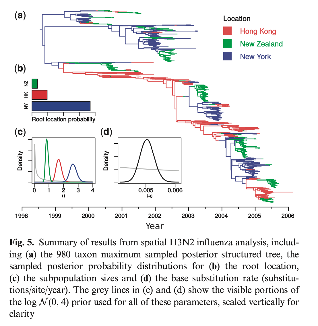
• Finally, they apply the model to a real dataset of global flu epidemics.
  •