Course notes: Machine Learning (Lee Hung-yi, 2016)

This post records the notes when I learnt the machine learning course from Lee Hung-yi.

0: Introduction of Machine Learning

The framework of machine learning can be summarized into three steps:

1. A set of functions (Model);
2. Goodness of function $f$ (build a function to evaluate the functions in step 1, e.g. Loss function);
3. Pick the best function (using training data (supervised learning, structured learning), or without training data (unsupervised training), or some combination (semi-supervised learning, transfer learning, reinforcement training)) and testing.

让我们朝着AI训练师的方向进发吧！

1: Regression

• Gradient descent: 只要可微分的function就可以用gradient descent找到local minima. 如果有多个参数, 就对每个参数(每一个dimension)做偏微分.But in linear regression, the Loss function is convex.
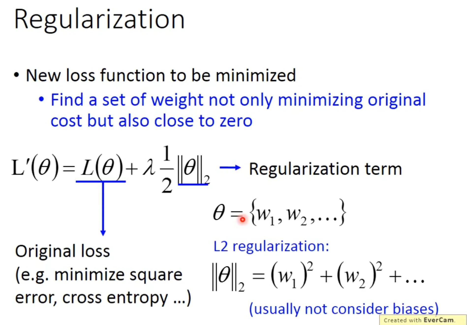
• Regularization: Redefined the loss function to make the function more smooth (the functions with smaller $w_i$ are better, therefore are insensitive to noise).
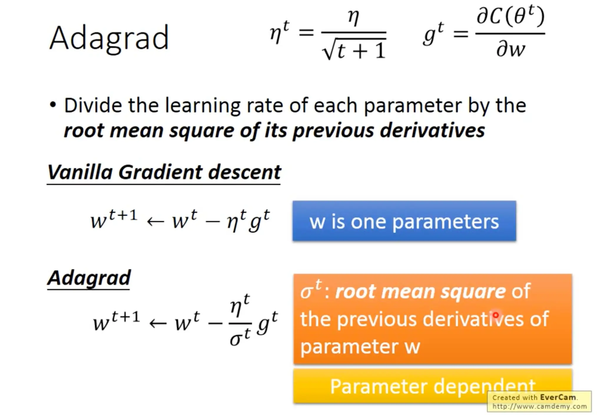
• Learning rate: we can specify customized learning rate for different parameters, e.g. Adagrad Optimizer.

2: Where dose the error come from

• There are two types of error : 1. from bias (the difference between the true function $\hat{f}$ and our estimated function $f^*$) and 2. from variance (the variance of the estimated functions).
  • Overfitting: Error from variance is too big. You should try to collect more training data, or use regularization.
  • Underfitting: Error from bias is too big. You should redesign your model (add more features or use a more complex model) to fit the training sets.
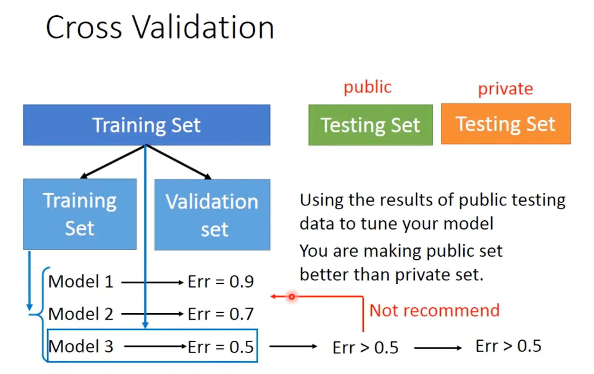
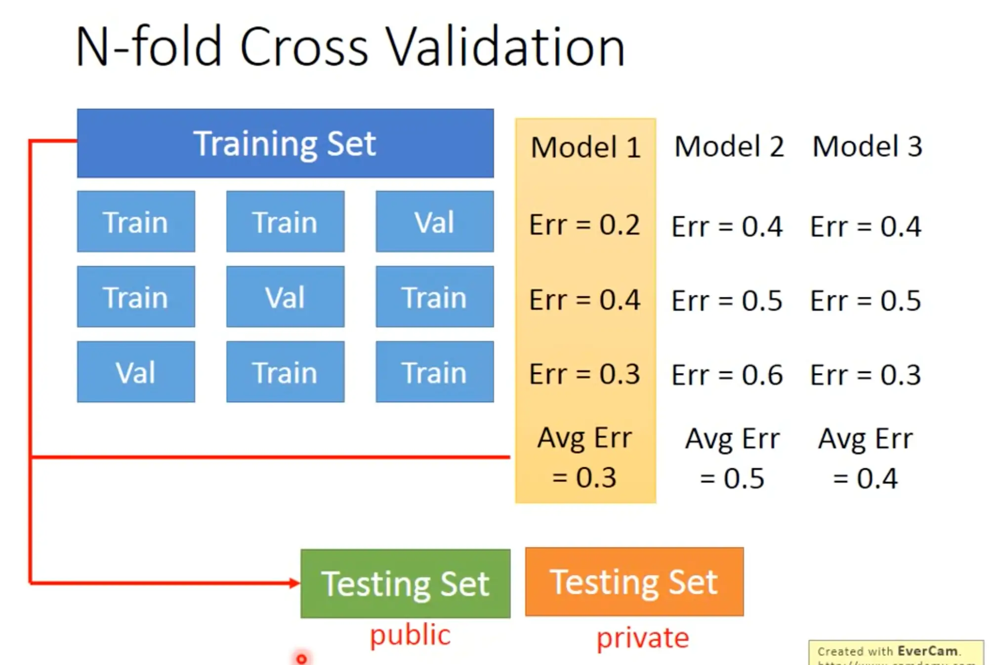
• Cross-validation: We should only use training set to choose your model, don’t cherry-picking with the testing set.

3: Gradient descent

Adaptive learning rate

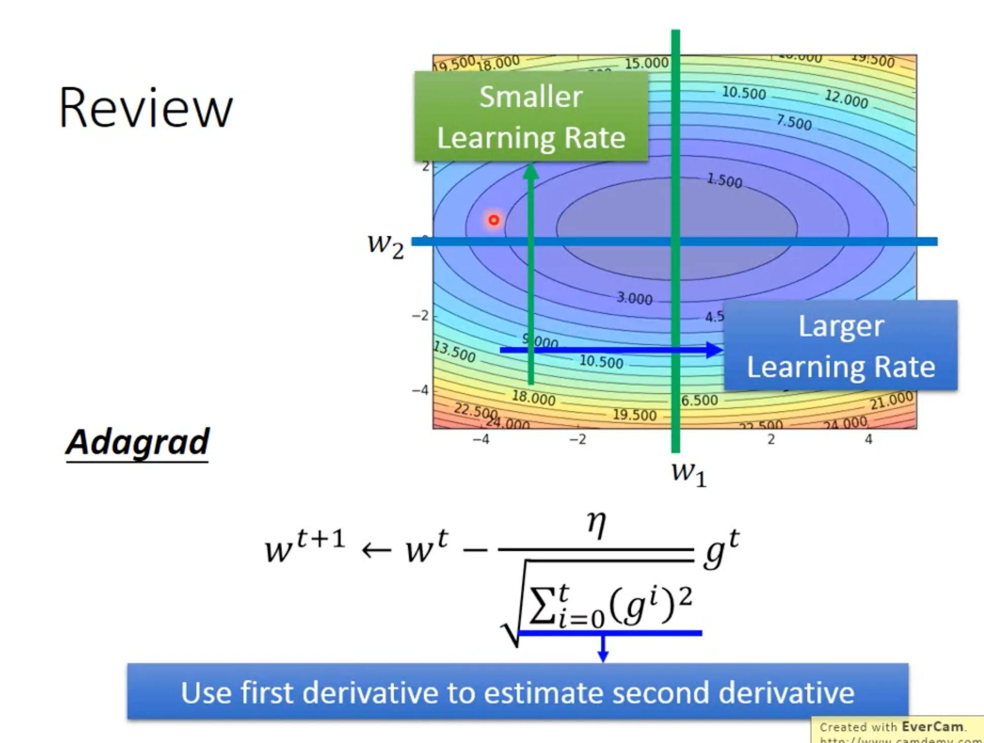
We can use adaptive learning rate to better approach the local minima. For example in the below figure, $\eta^t$ depends on the number of epochs $t$, and $\sigma^t$ depends on (all) the previous derivatives.

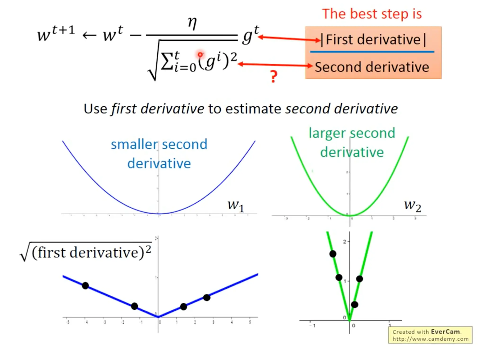
The denominator in adagrad formula estimates the second derivative of the gradient. We need to account for the second derivative because the best step should also consider the second derivative (see below: although the points in $w2$ have bigger first derivatives than data points in $w1$, they in fact are more close to the local minima).

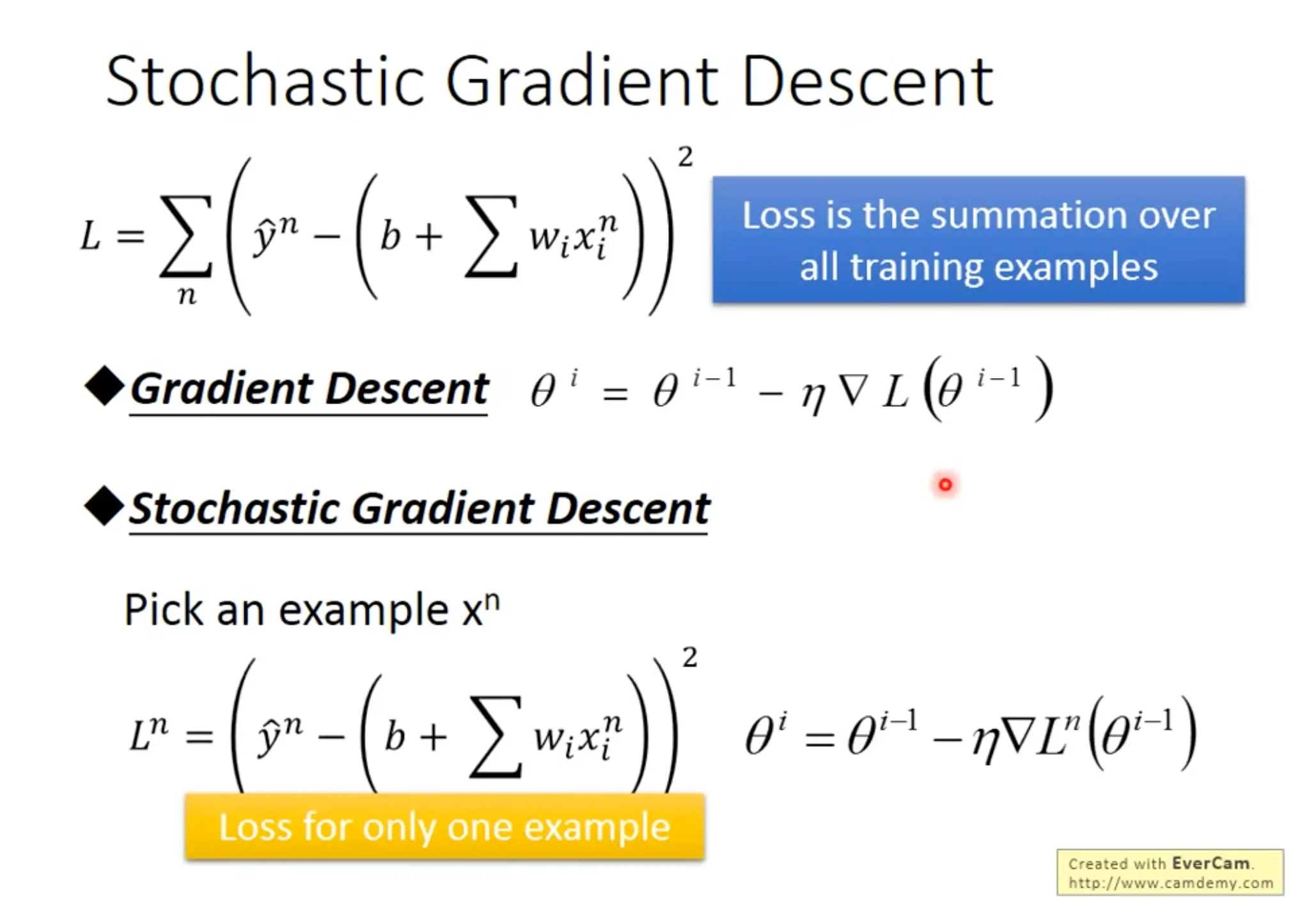
Stochastic gradient descent

Loss for only one sample, the advantage is it can update very frequently.

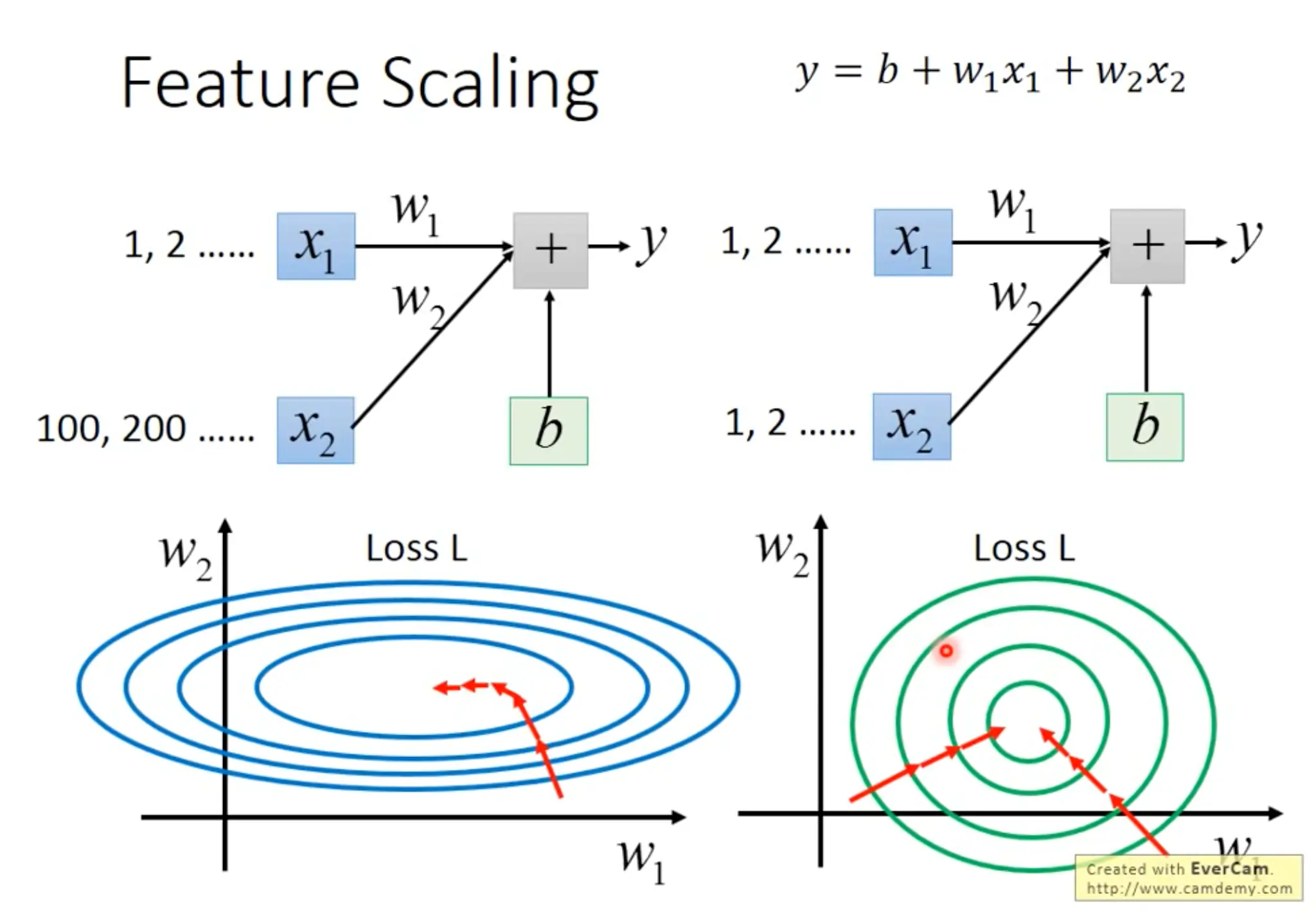
Feature scaling

Make different features have the same scaling will help finding the local minima more efficiently.

4. Classification

In classification problems, the outputs are class/categories.

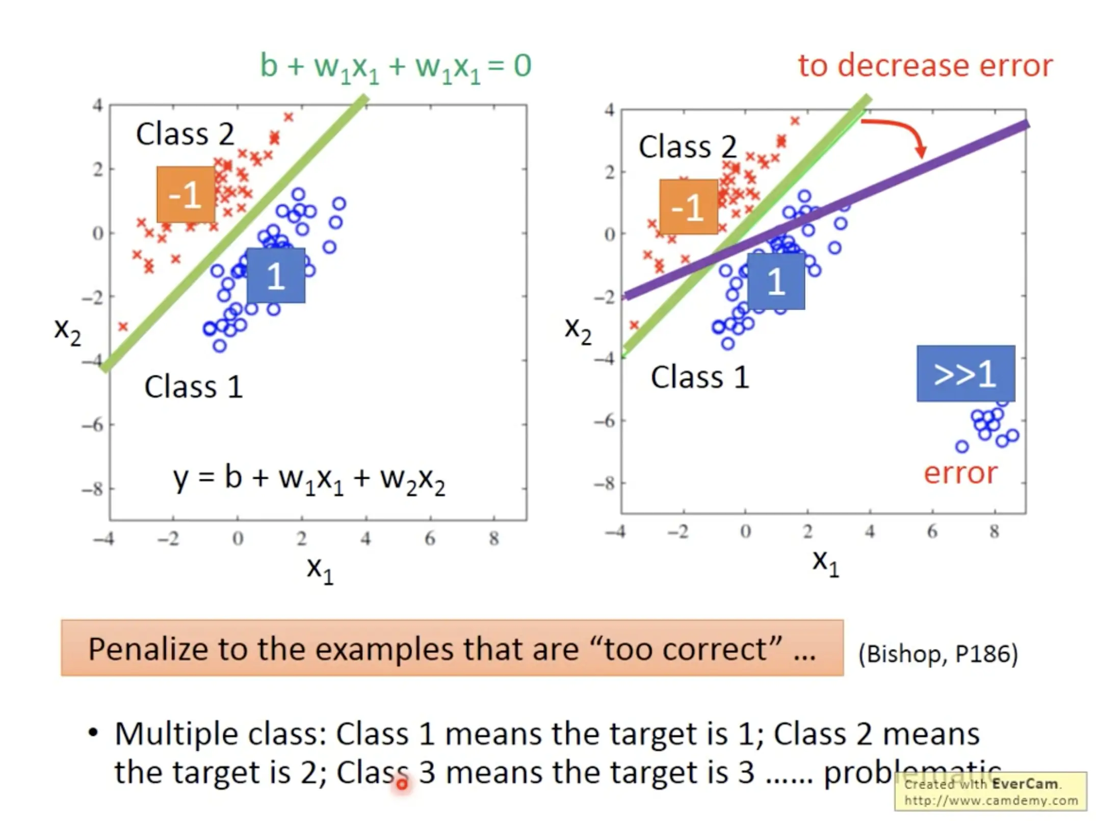
Naive regression

To solve a classification problem, one way (probably in instinct) is to use the regression. Specifically, you can label one class as $1$ and the other class as $-1$, then find the best parameters $w_1$ and $w_2$ in the model $y=b+w_1x_1+w_2x_2$. However, there are some problem with this naive approach, that it is sensitive to outlier values, and it is hard to deal with multiple classes:

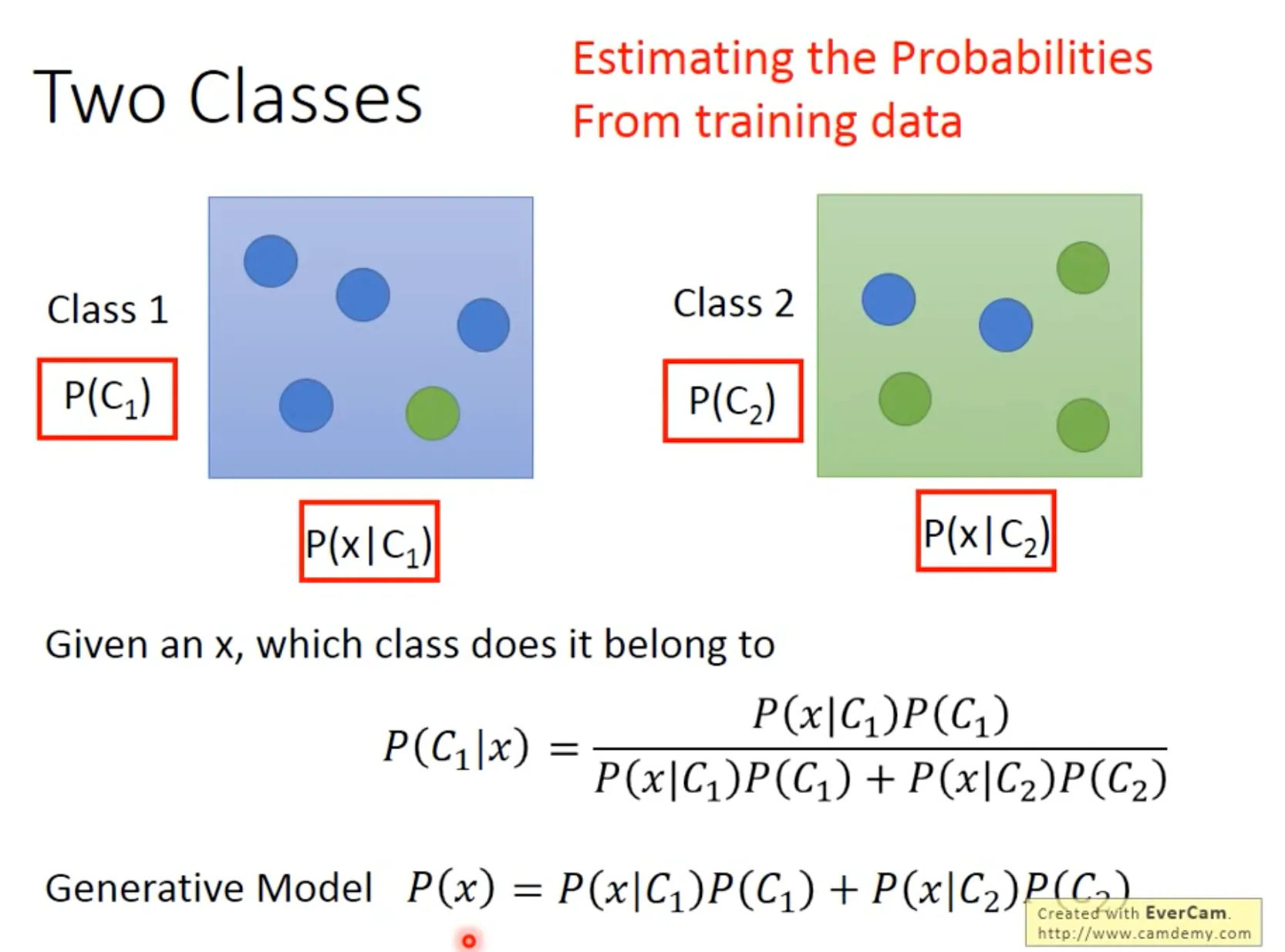
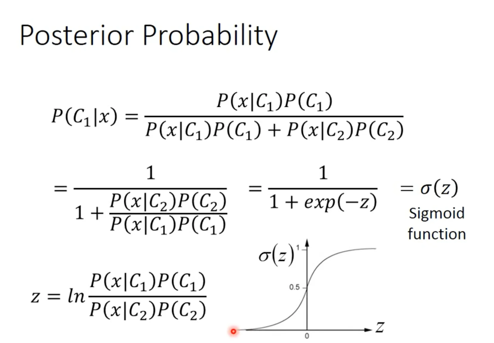
Probability generative model

与生成模型(generative model)对应的是决断模型(descrimintive model). 类似regression, SVM这样的模型属于决断模型.而另一种思路是生成模型, 即生成每个class的概率分布, 然后对比新的feature在每个class的概率分布里面的可能性(e.g., $P(x|C_1)$)的大小.

三步建立概率生成模型

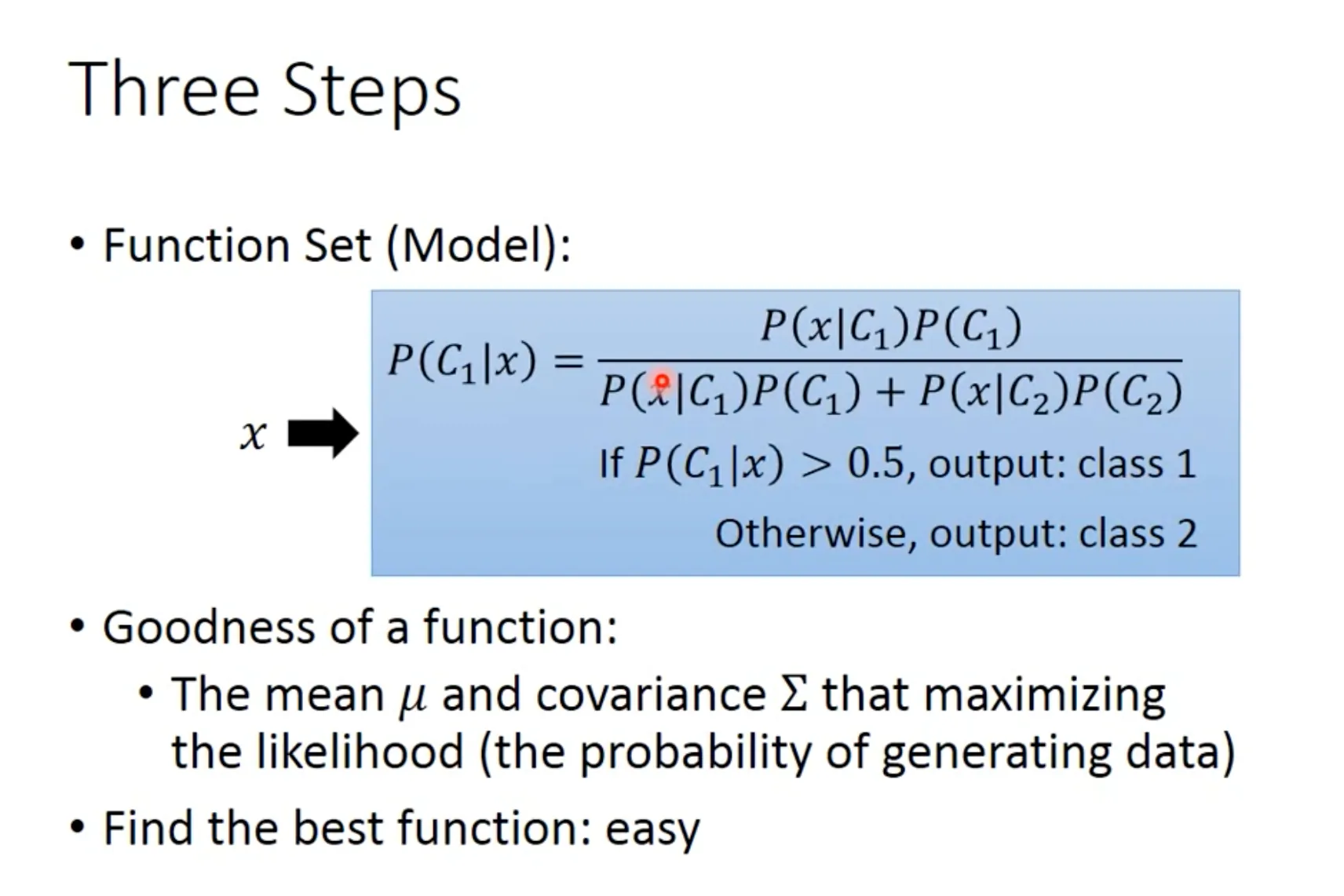
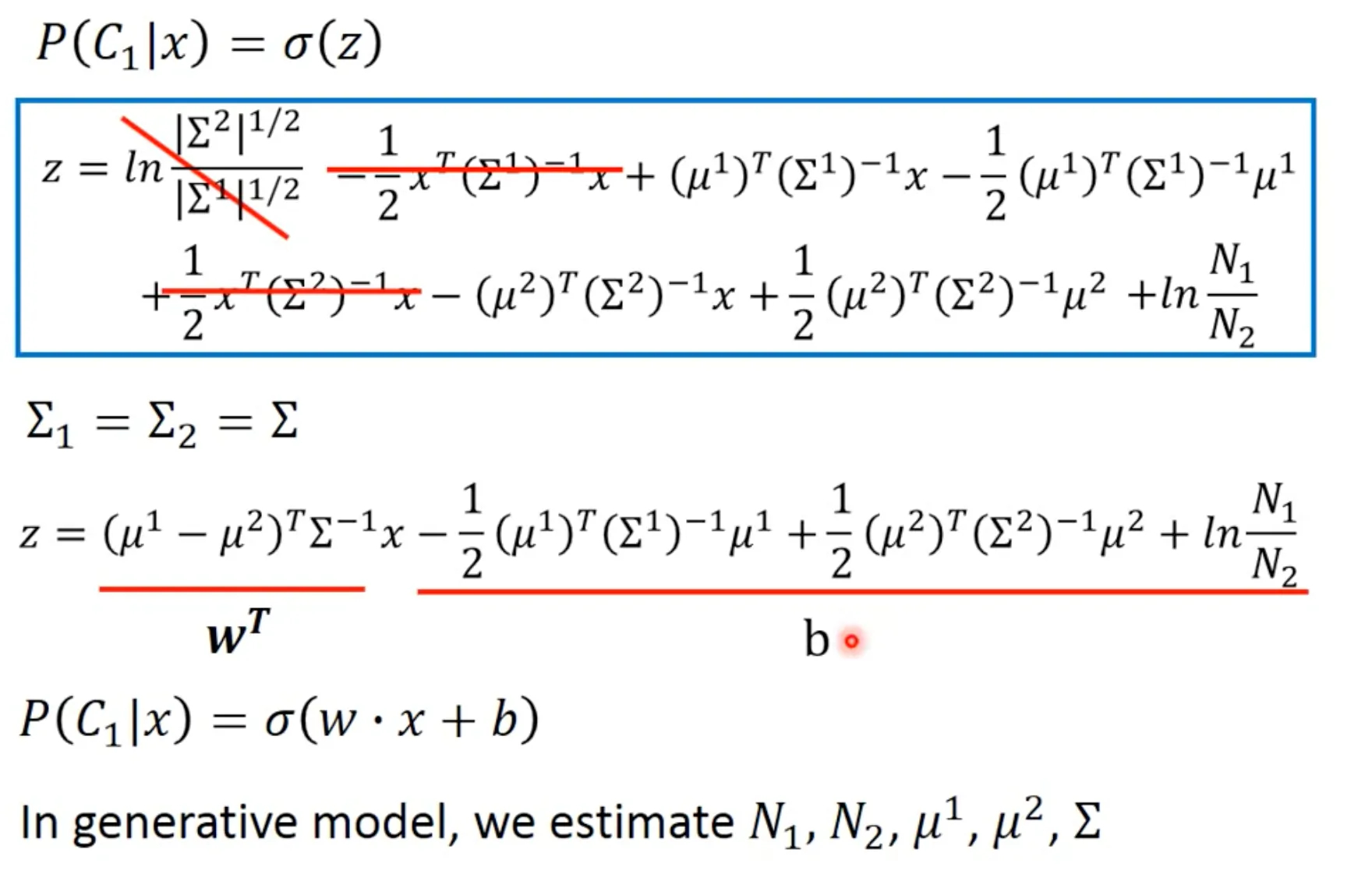
如果不同参数之间是independent的, 这种情况下构成一个Naive Bayes Classifier. 而当不同的class的概率分布share同一个covariance matrix的时候, 这是一个”linear model” (2-D的时候, 判别线为直线). 2-D下, 当$\Sigma_1=\Sigma_2$时, 其linearity可见下面的推导:

中间步骤省略

5. Logistic Regression

Logistic Regression可以跟上面的Probability generative model里面的特殊情形(shared covariance matrix)联系起来,但logistic regression不假设任何概率分布. 本质上是一个通过sigmod function连接的linear regression.

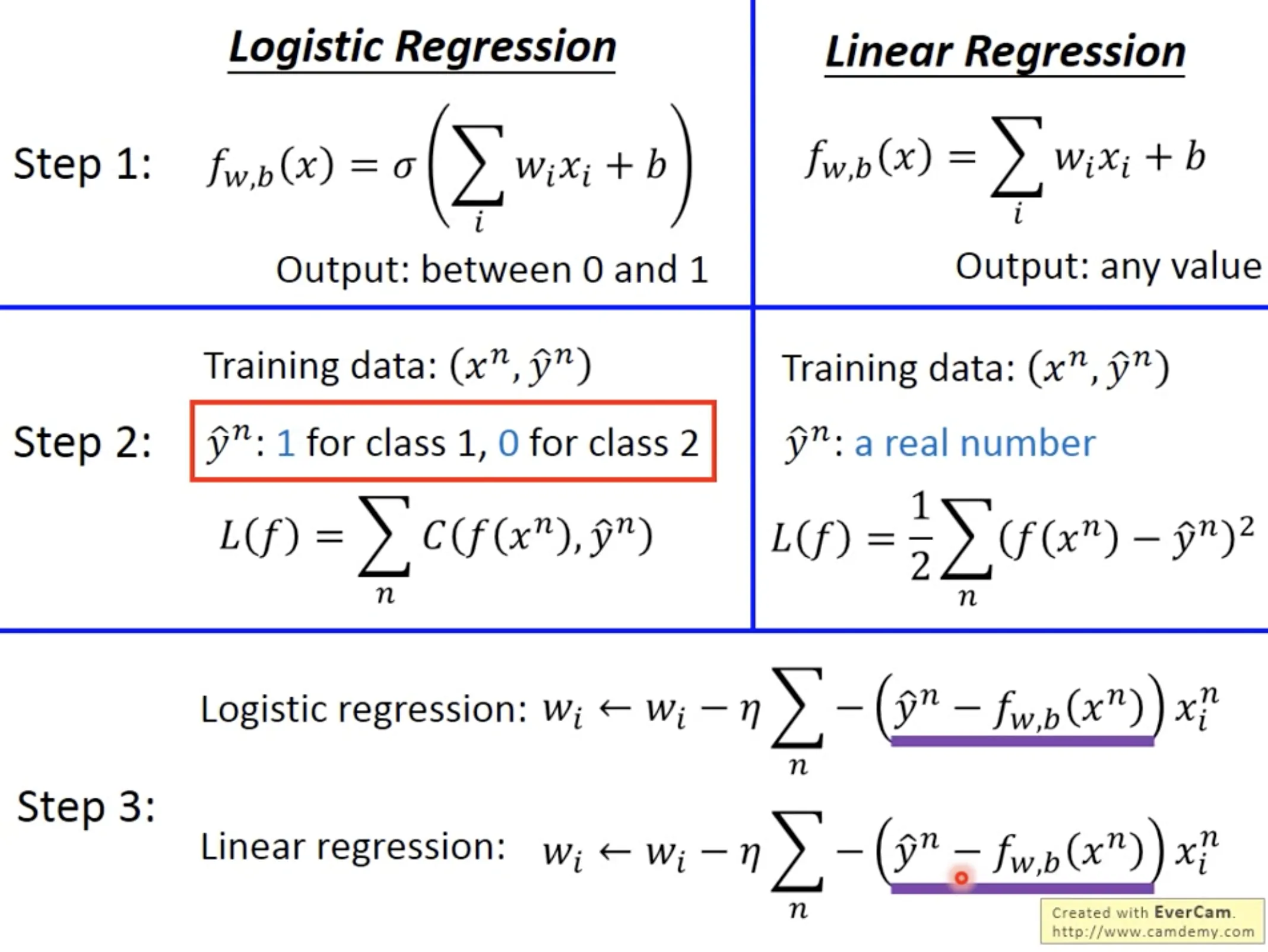
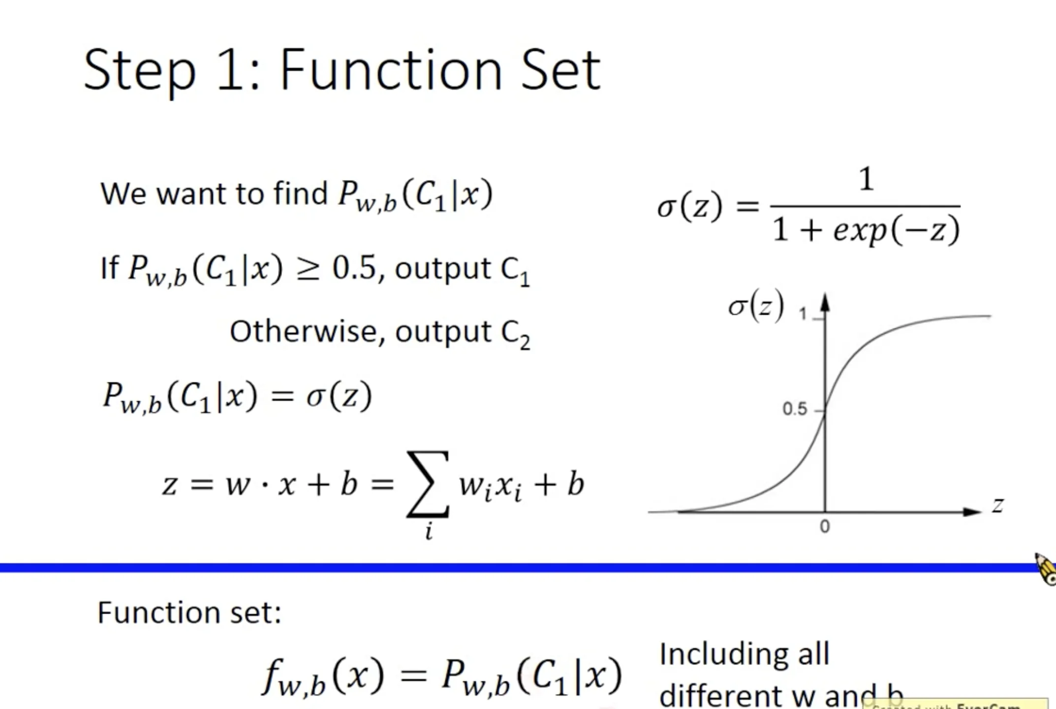
Step 1: Function set

The posterior probability $P(C_1|x_1)$ is a function set, which contains all combination of parameters $w$ and $b$.

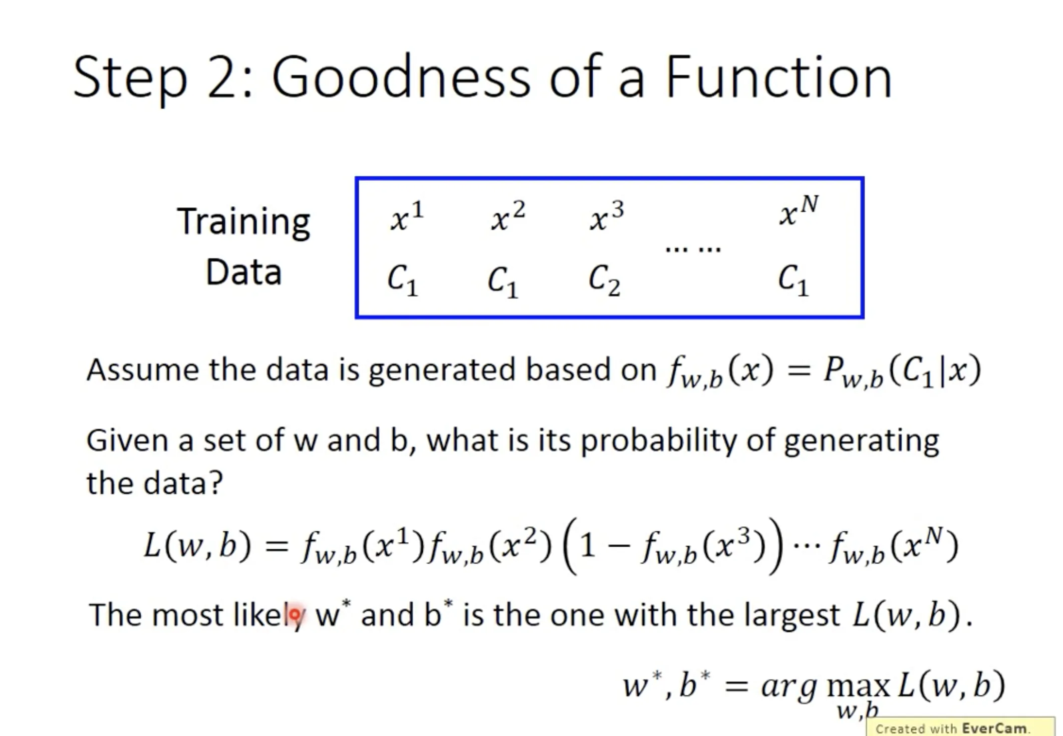
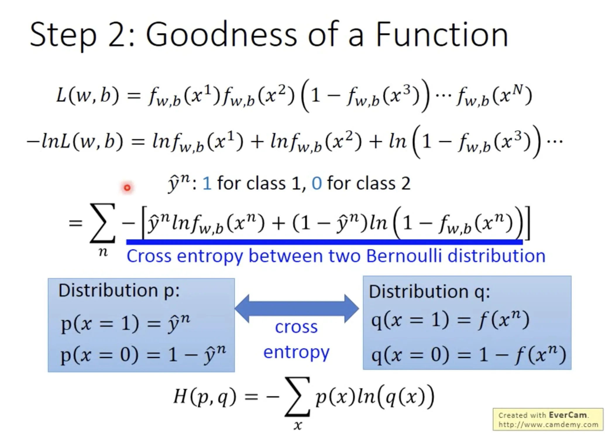
Step 2: Goodness of the function

Using maximal likelihood, we can find the best function. The loss function of Logistic Regression is the sum of cross entropy between $f(x^n)$ and $\hat{y}^n$.

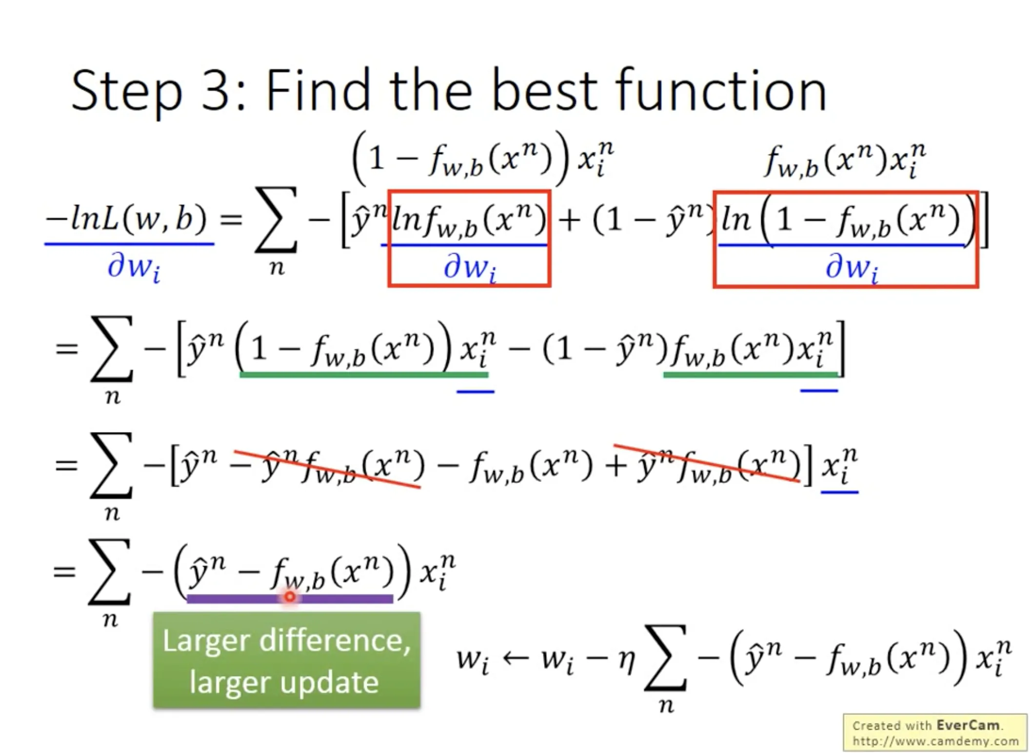
Step 3: Find the best function

对$w_i$和$b_i$取偏微分, 用gradient descent.

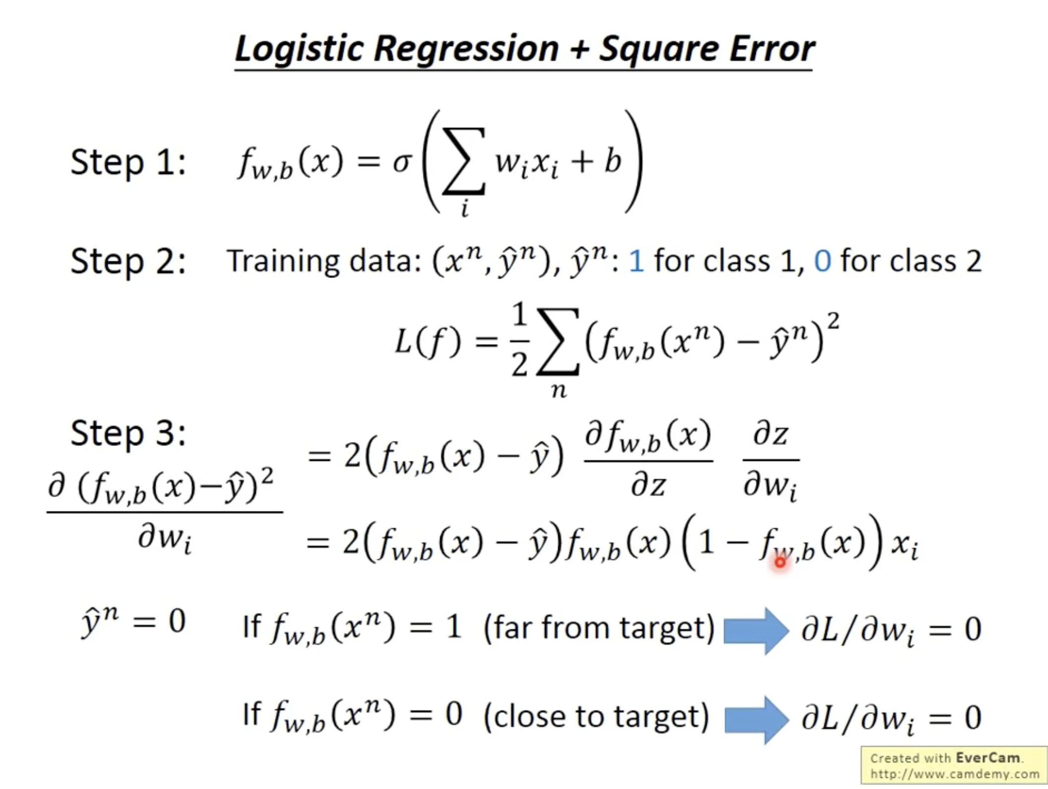
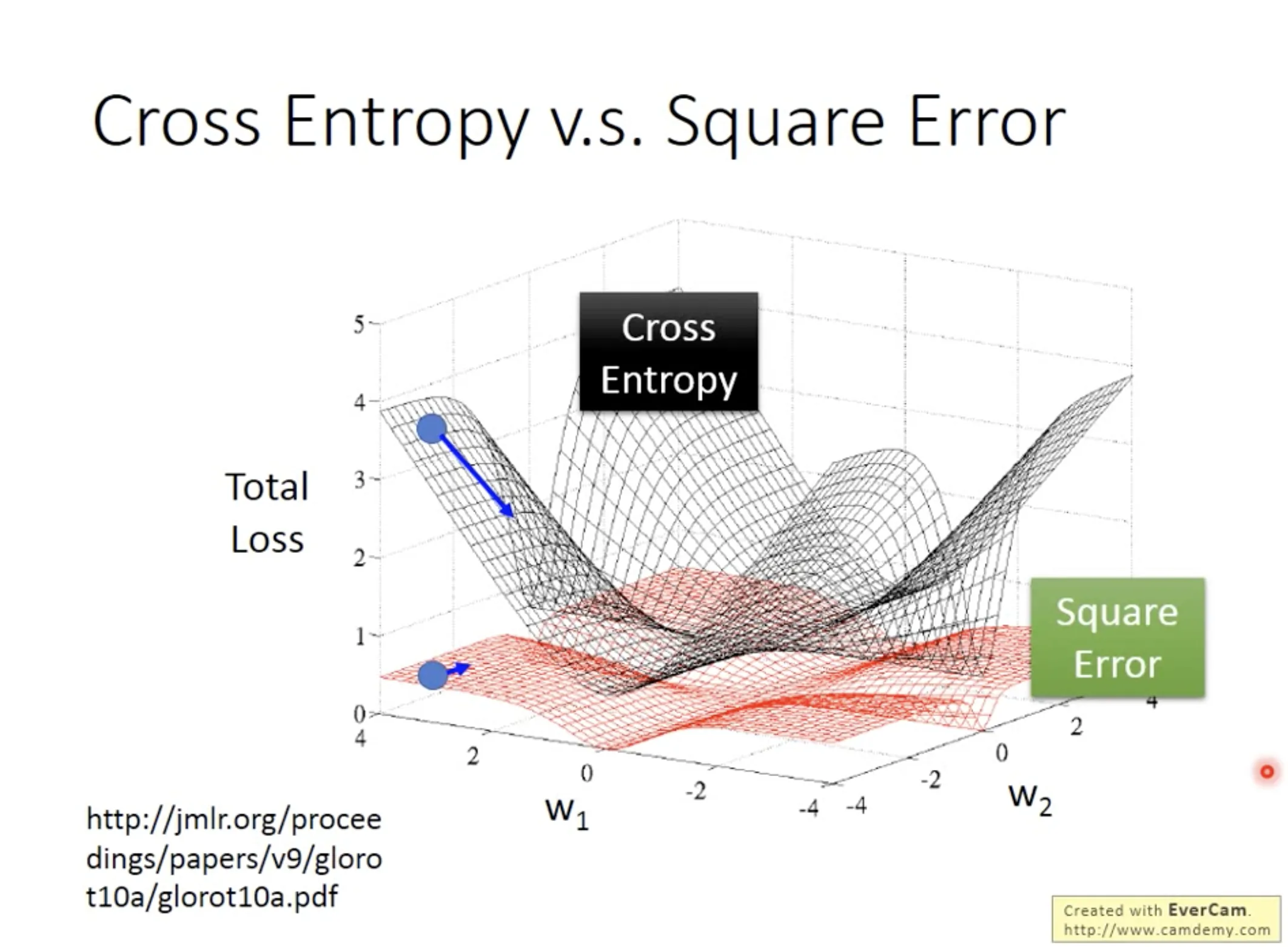
Why can’t we use square error as the loss function

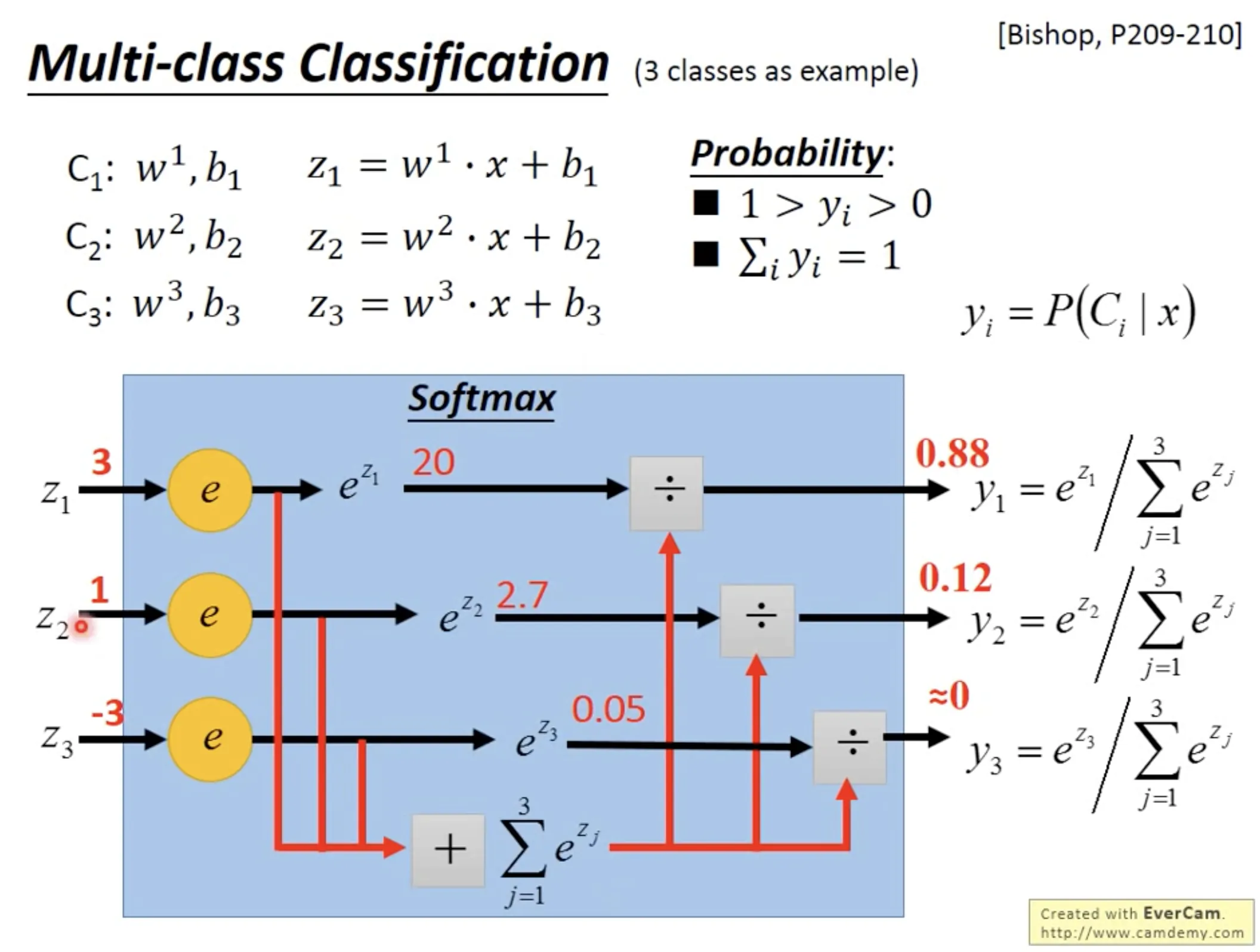
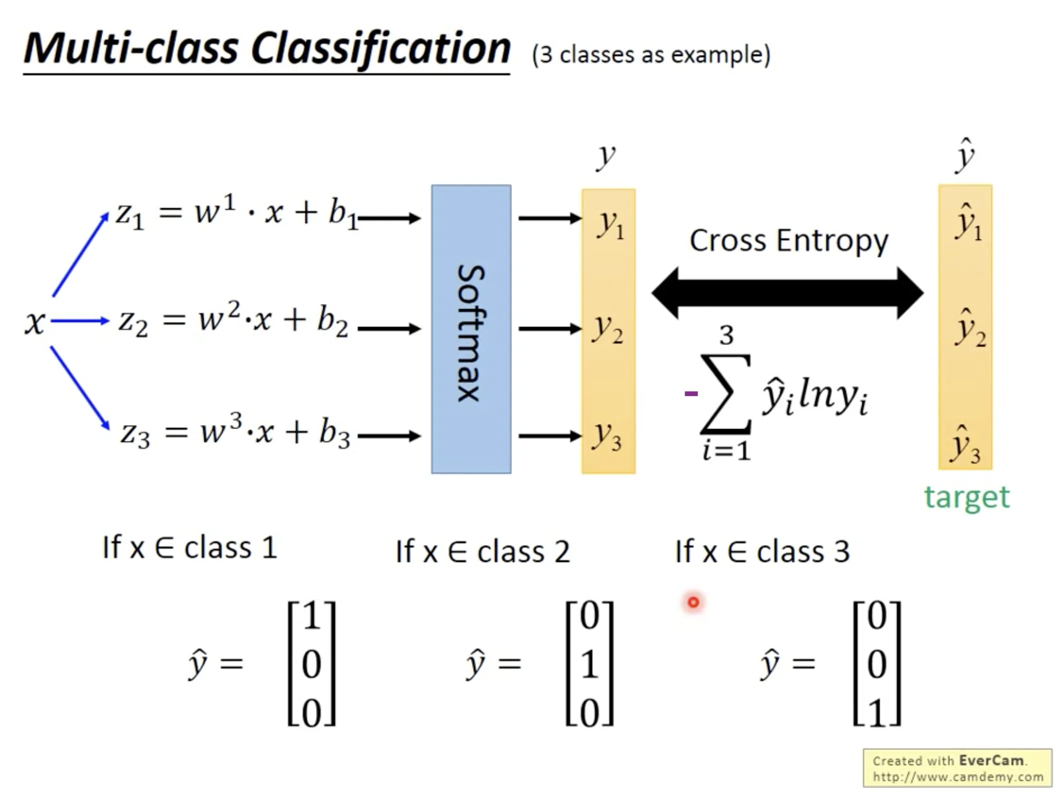
Multi-class classification

Limitation of logistic regression

The boundary is linear, thus it can not fit into some data. We can use feature transformation to cope with this. Specifically, when we can cascade logistic regression models, then it will be a simple neural network!

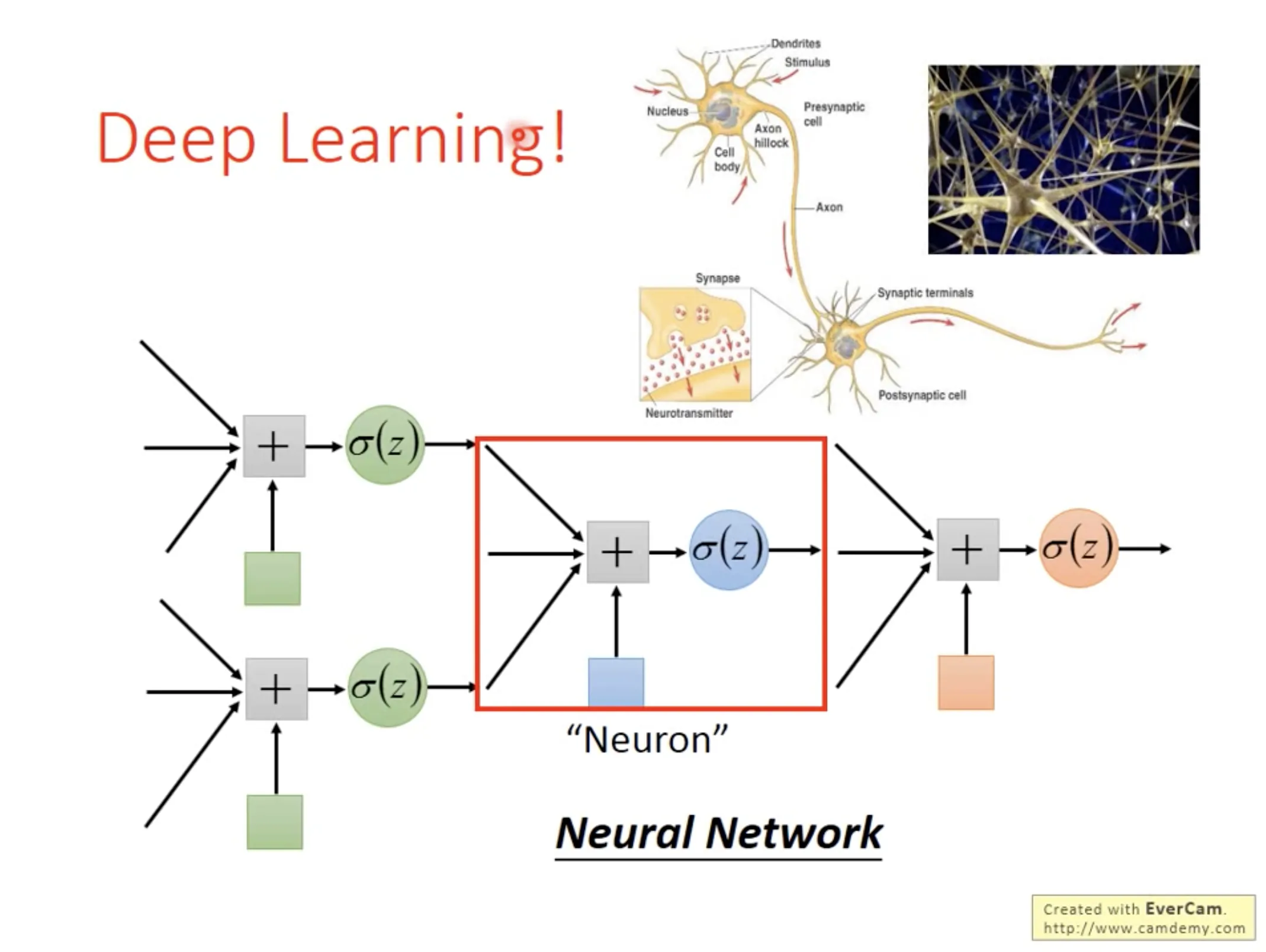
6. Brief introduction of Deep Learning

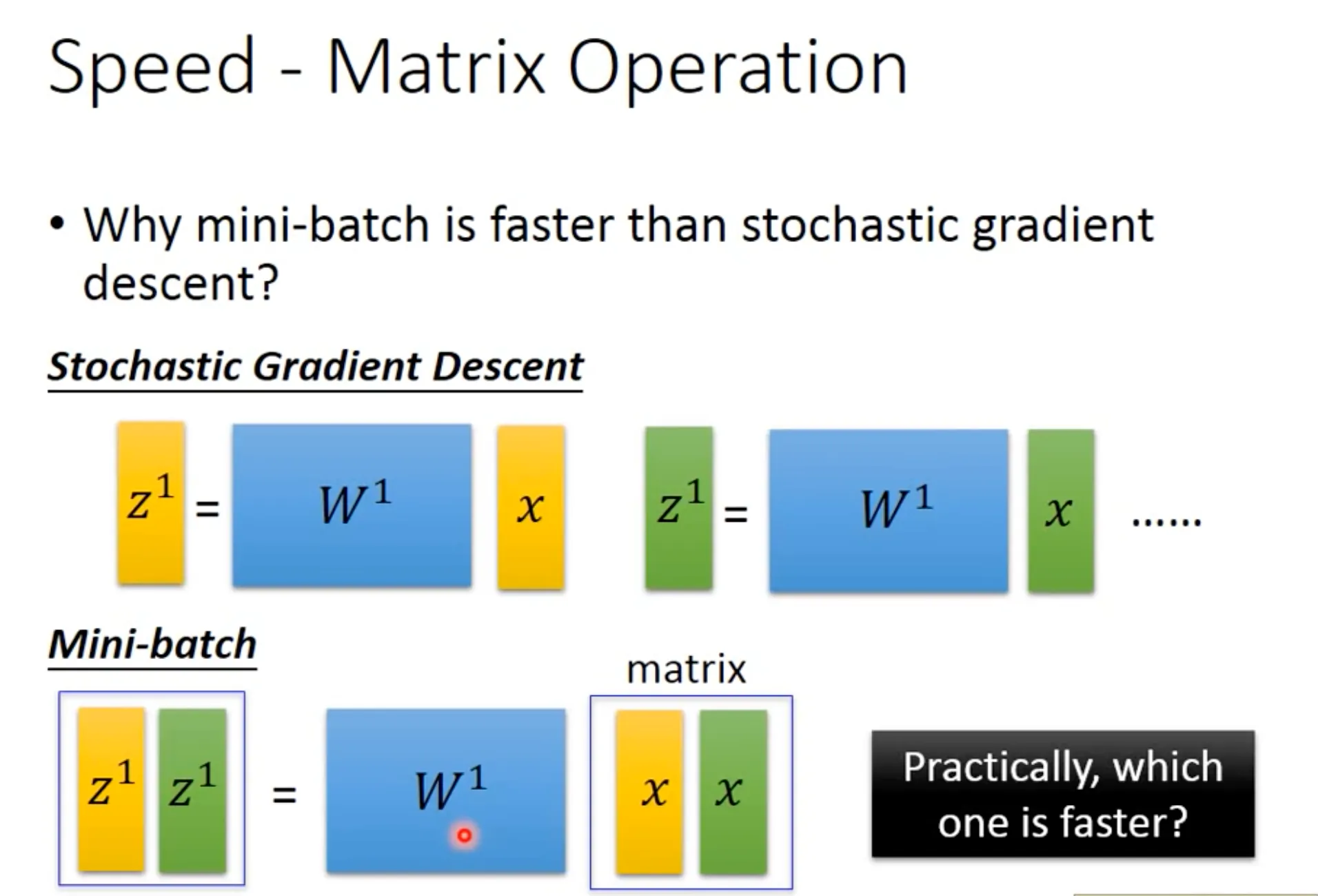
Neural network是一连串的matrix的operation, 所以用GPU可以方便计算.

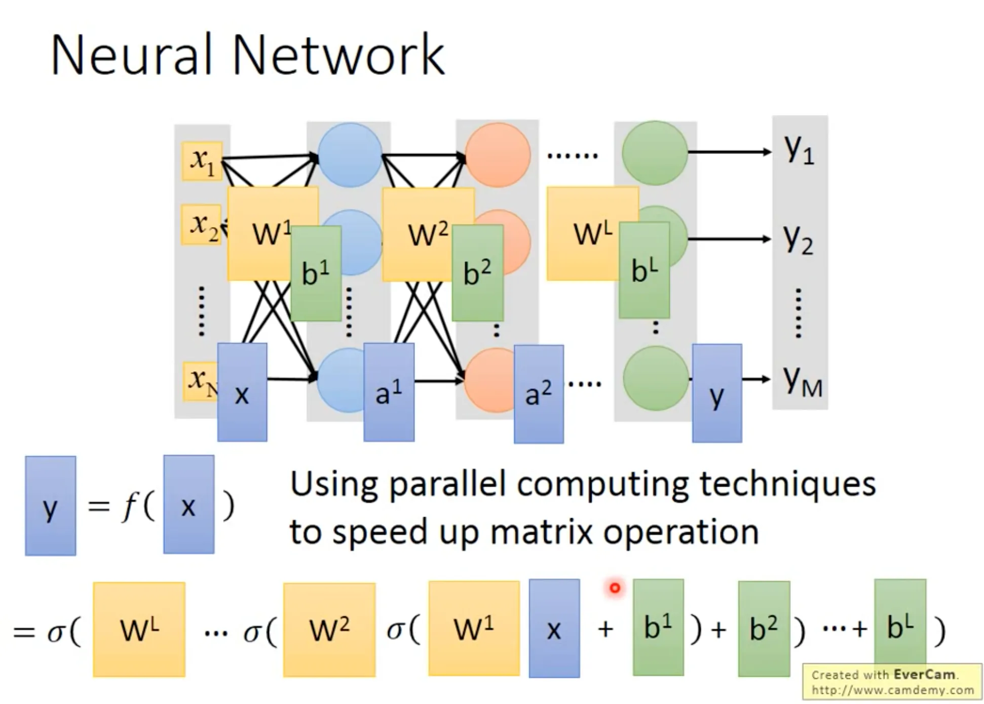
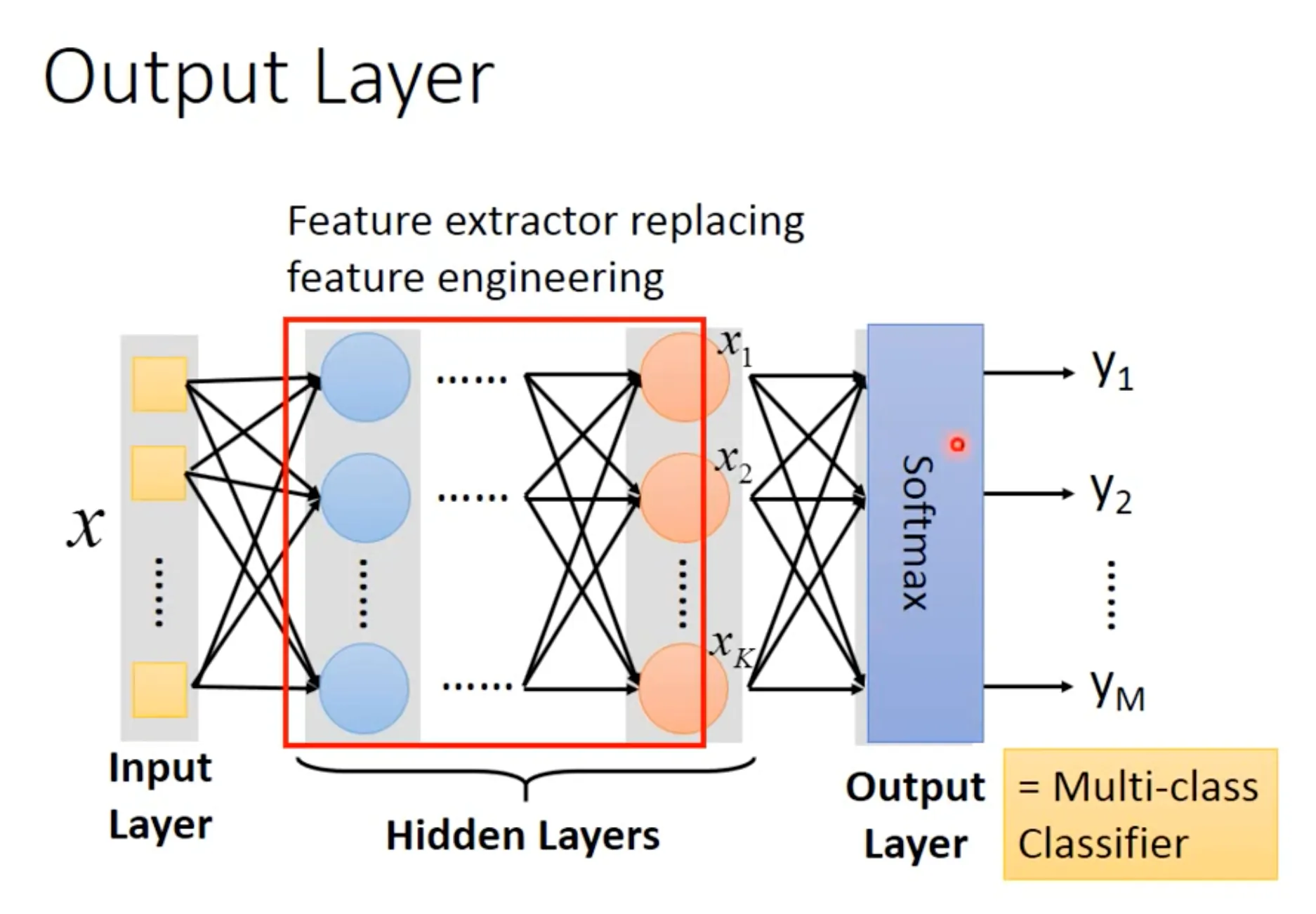
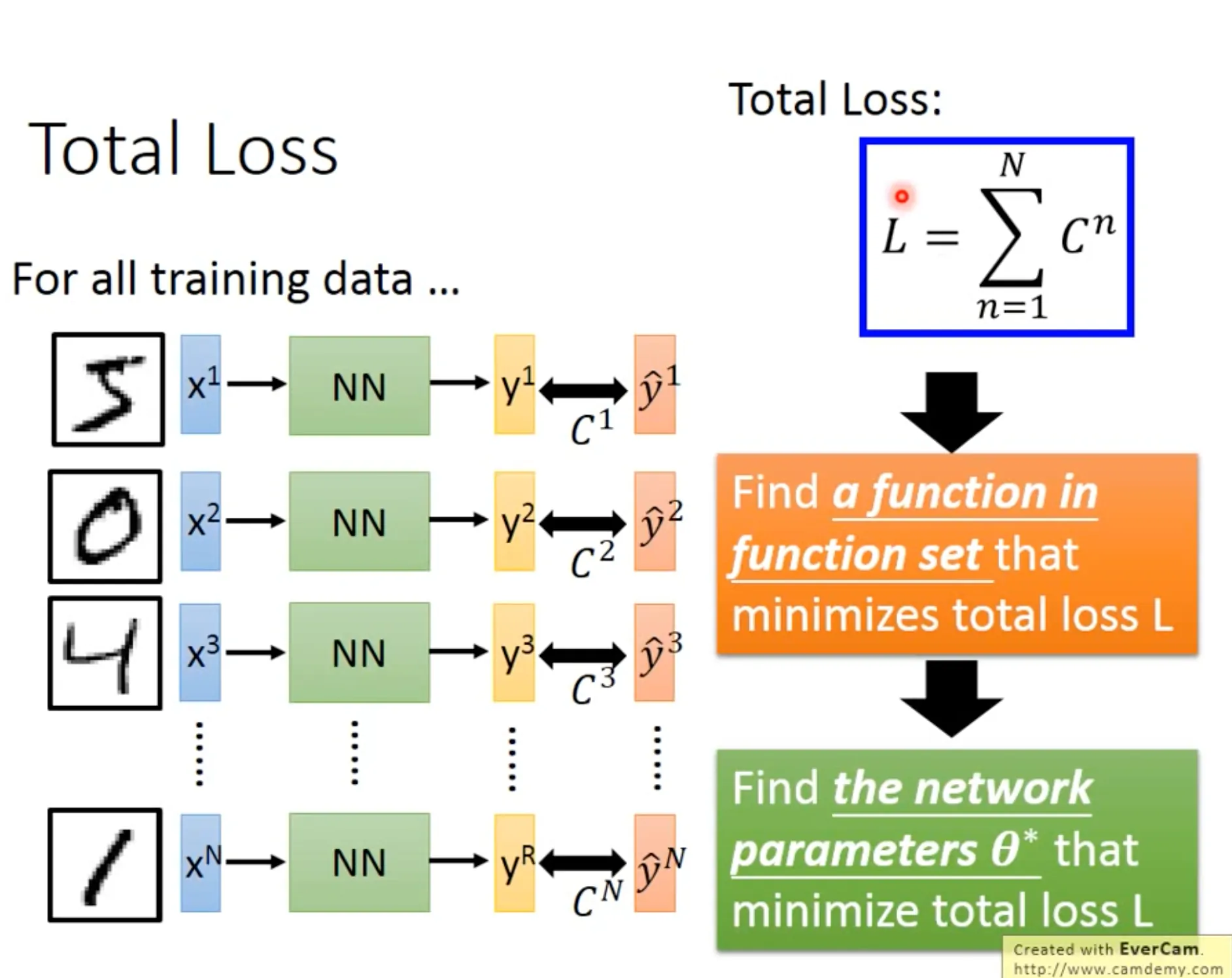
Neural network的中间层可以视为feature transformation的过程, 最后的output layer一般接一个softmax, 即可作为multi-class classifier. Loss function也和multi-class classification的时候一摸一样, 计算$f(x^n)$ and $\hat{y}^n$ 的cross entropy即可.

Find the best function的过程也是一样, 用gradient descent即可. Backpropagation 是一个有效算微分的方法.

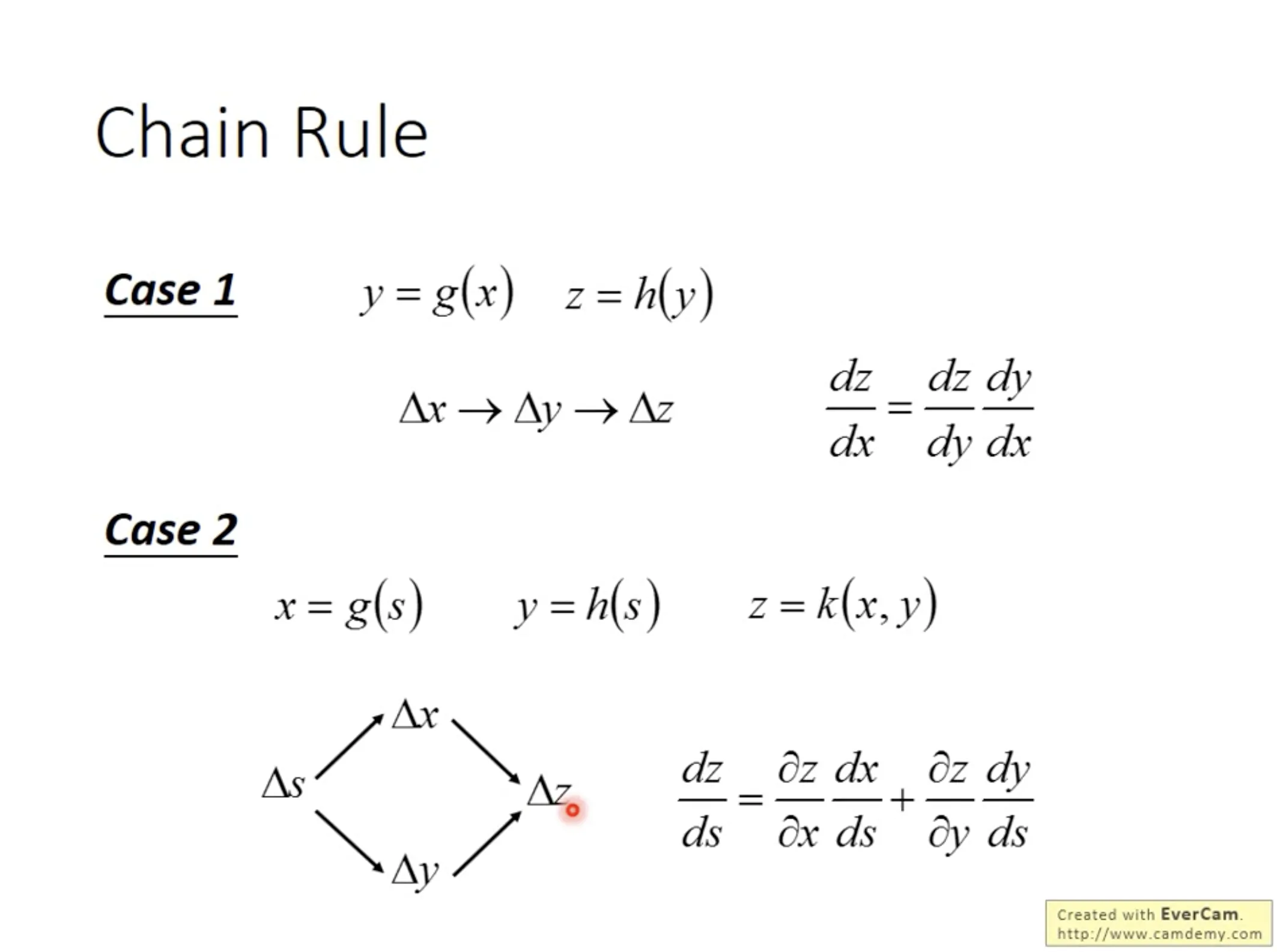
7. Backpropagation

Backpropagation是一种用来高效求微分的方法. 先复习一下链式法则;)

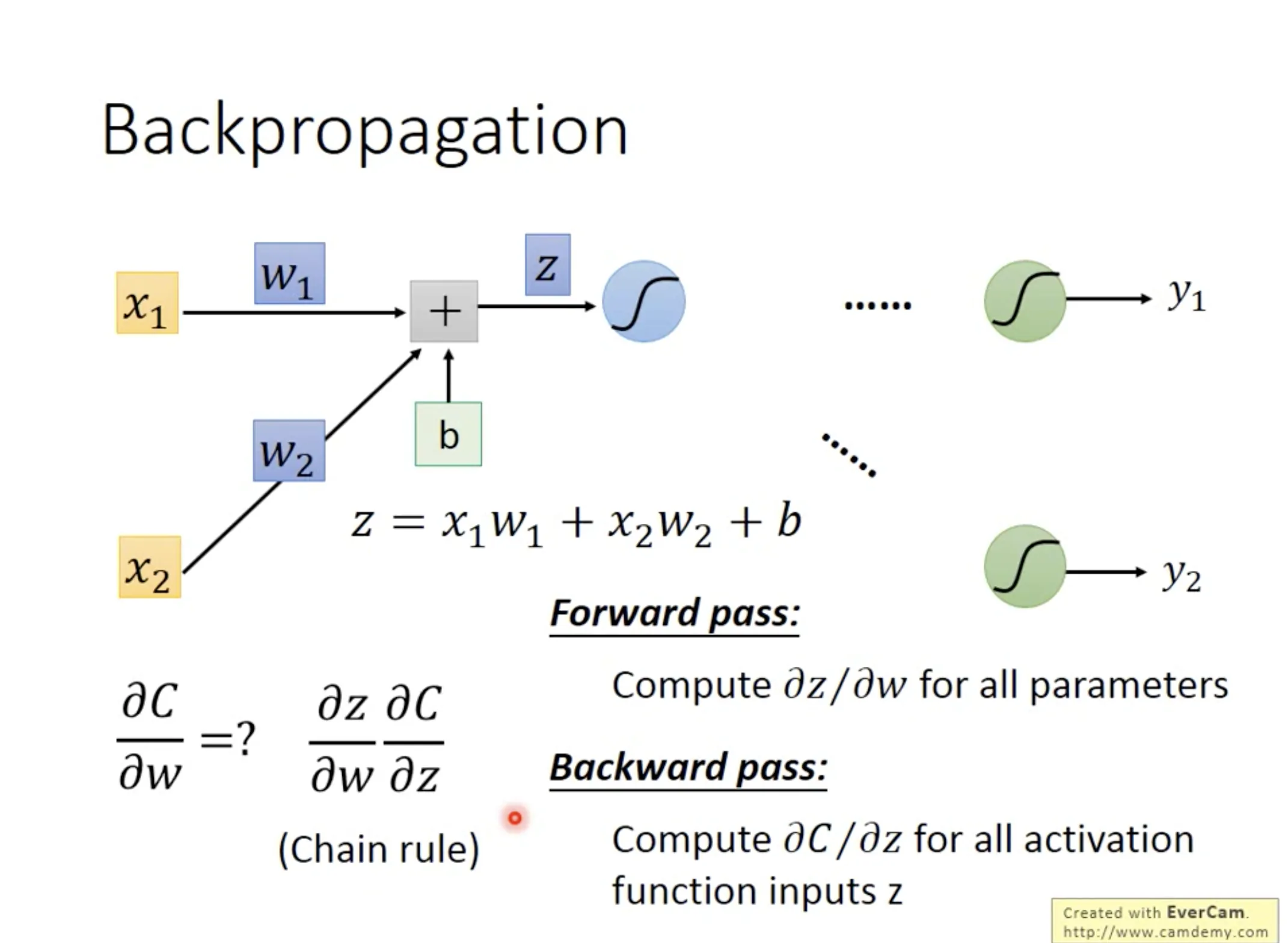
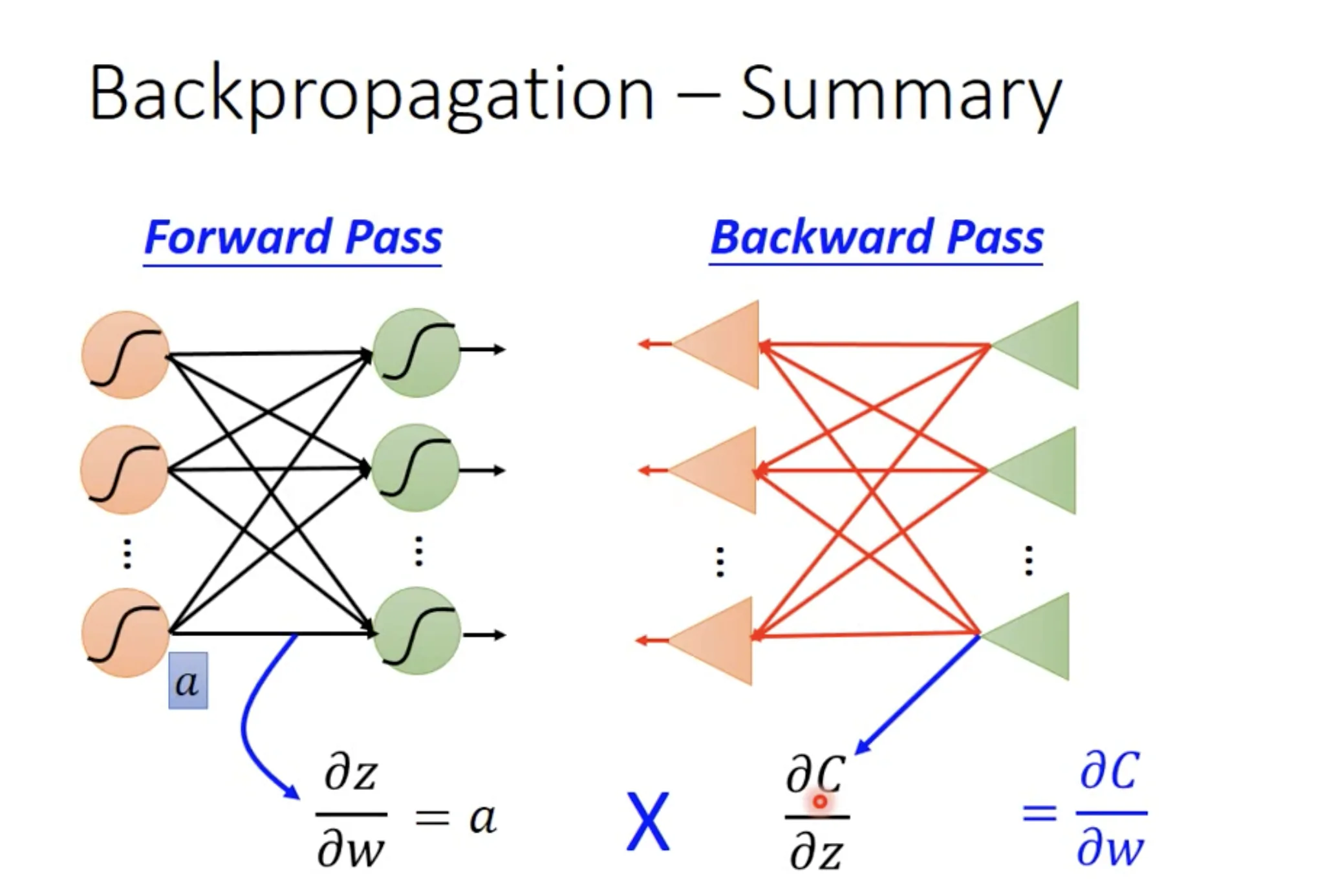
$\frac{\partial{C}}{\partial{w}}$可以由$\frac{\partial{C}}{\partial{z}}$ (calculated by backward pass) 和$\frac{\partial{z}}{\partial{w}}$ (calculated by forward pass)计算.

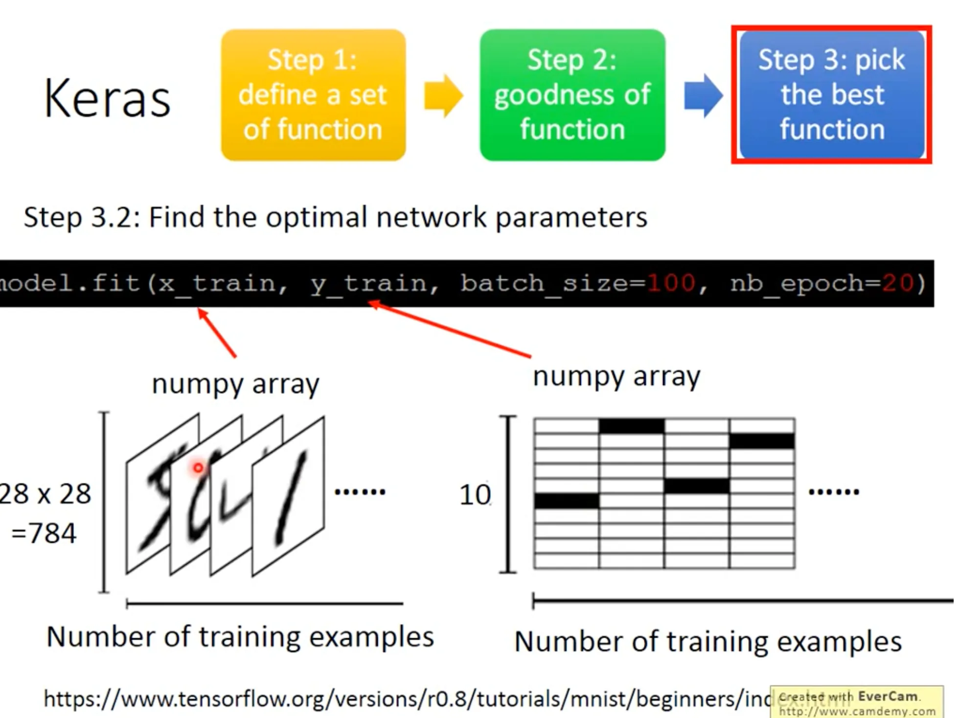
8. Keras

为什么不是batch size越大越好？ 请注意neural network的问题并不少covex的, 你如果不添加一点随机性(用小一点的batch size), 那么模型很容易一下子就陷到local minima了.随机性是必要的, 以便于离开一个saddle point或不是很深的local minima. (这跟做决策一样, 既然我们无法预测未来, 我们可能需要一点随机性:smirk:)

GPU加速的秘诀在于用mini batch的时候, 跟用stochastic gradient descent(一个sample一个batch, 计算速度几乎是一样的.

9. Tips for training DNN

在训练神经网络的时候, 会遇到两种情形需要我们去调整模型: 1. 训练集的拟合不好; 2. 测试集效果太差.

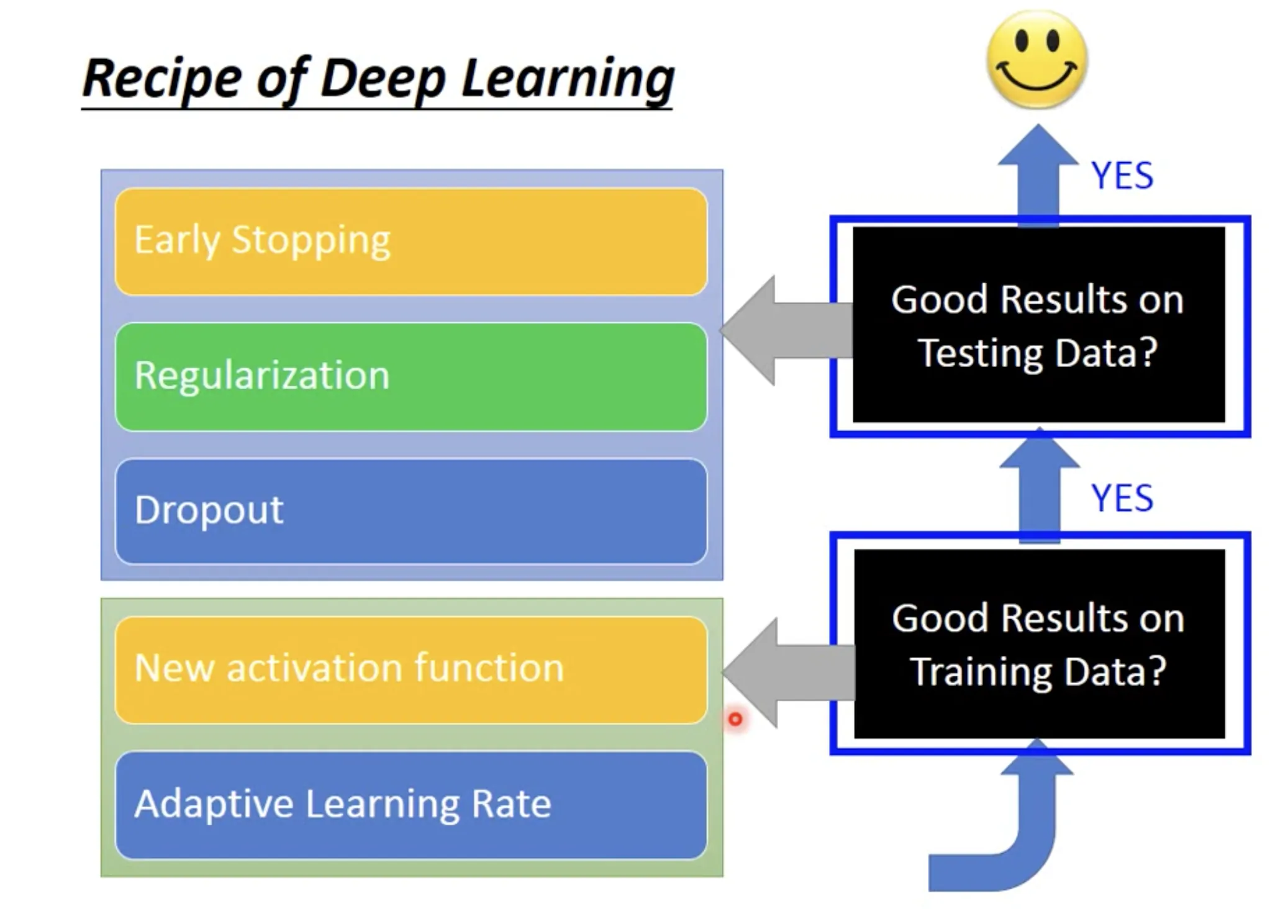
Improve fitting on training data

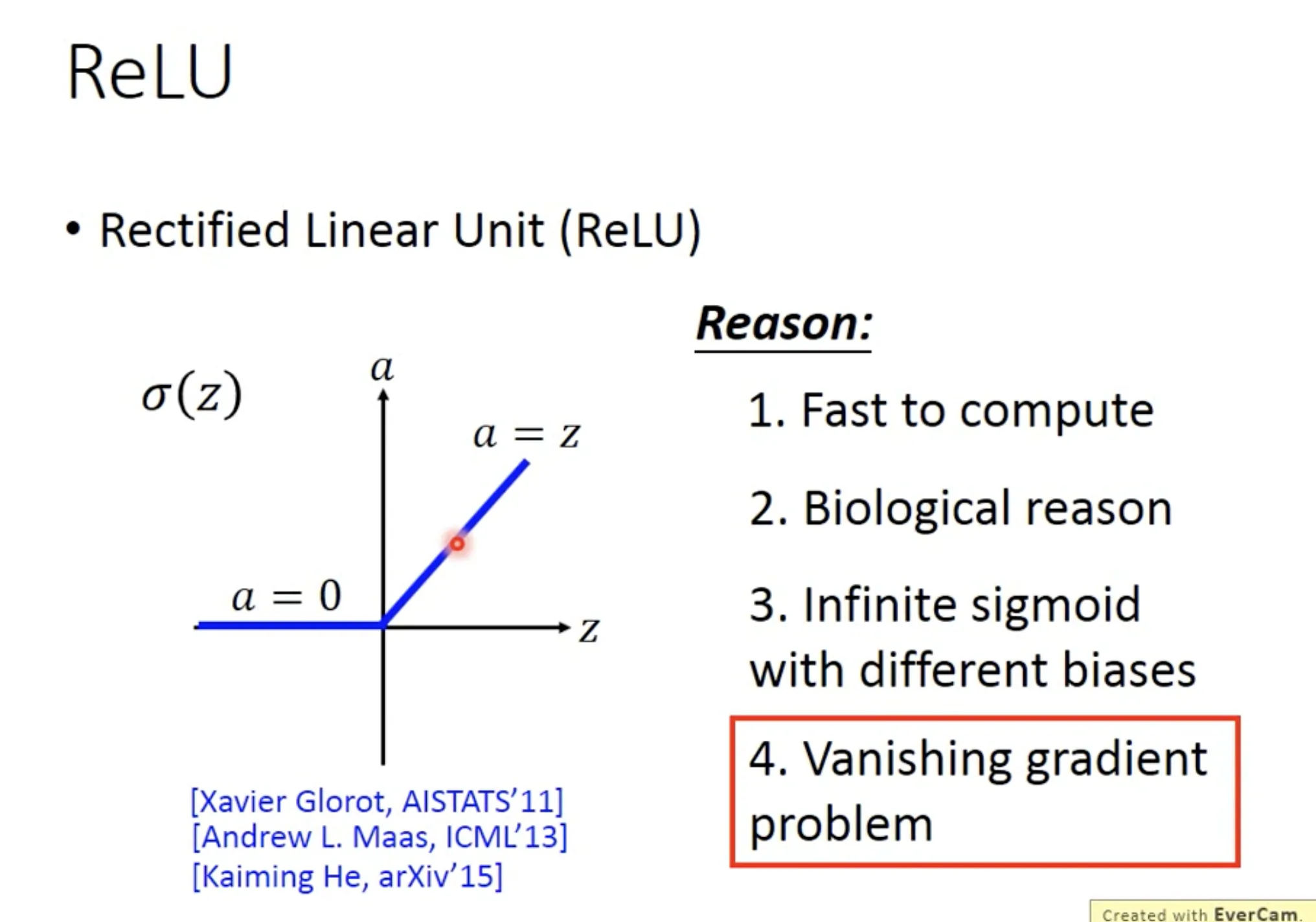
Change activation function

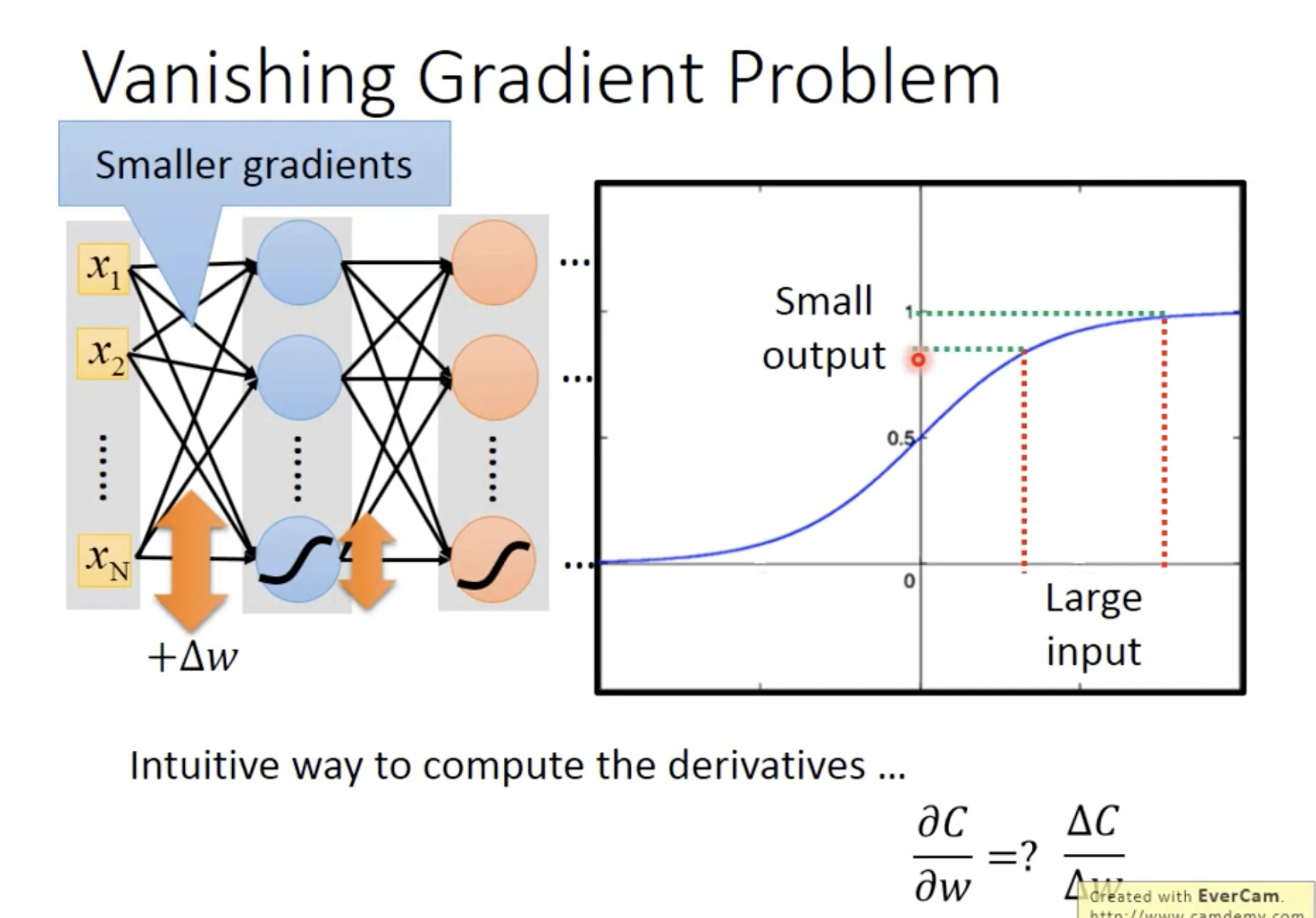
在用sigmod function做activation function的时候, 如果layer多了, 会遇到vanishing gradient problem. 它的意思是, 前面layer的参数$w$对loss function的微分会很小.

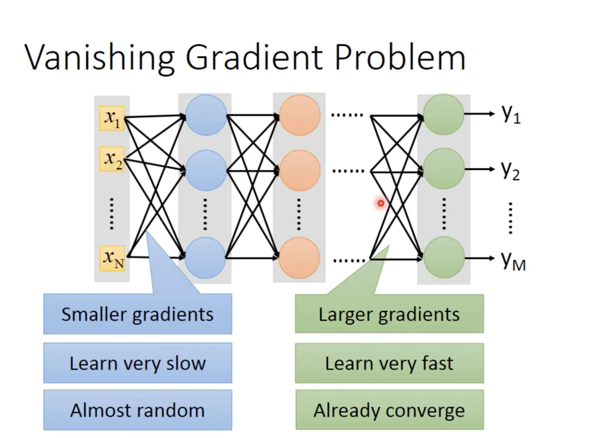
一个直觉的理解是, 在前面的layer里面, 即使有很大的参数变化$\Delta{w}$, 由于sigmod function的性质, 它的作用在传递过程中, 是不断减弱的. 从而使backpropagation回来之后的gradient相应地减少.

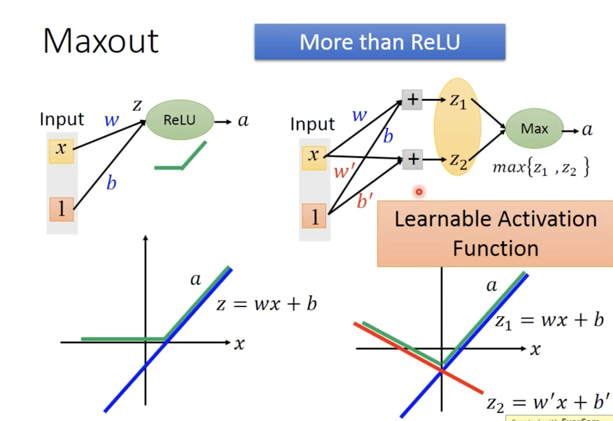
有一些比较线性的activation functions可以解决这个问题, 比如reLU和maxout. reLU可以表示为Maxout的一种特殊形式, 意味着maxout会更加versatile, 它也是一个learnable的activation function.

Adaptive learning rate

Adagrad之前已经提过, 可以用来给每个参数赋予不同的learning rate (传递这个参数之前所有的gradient的影响).

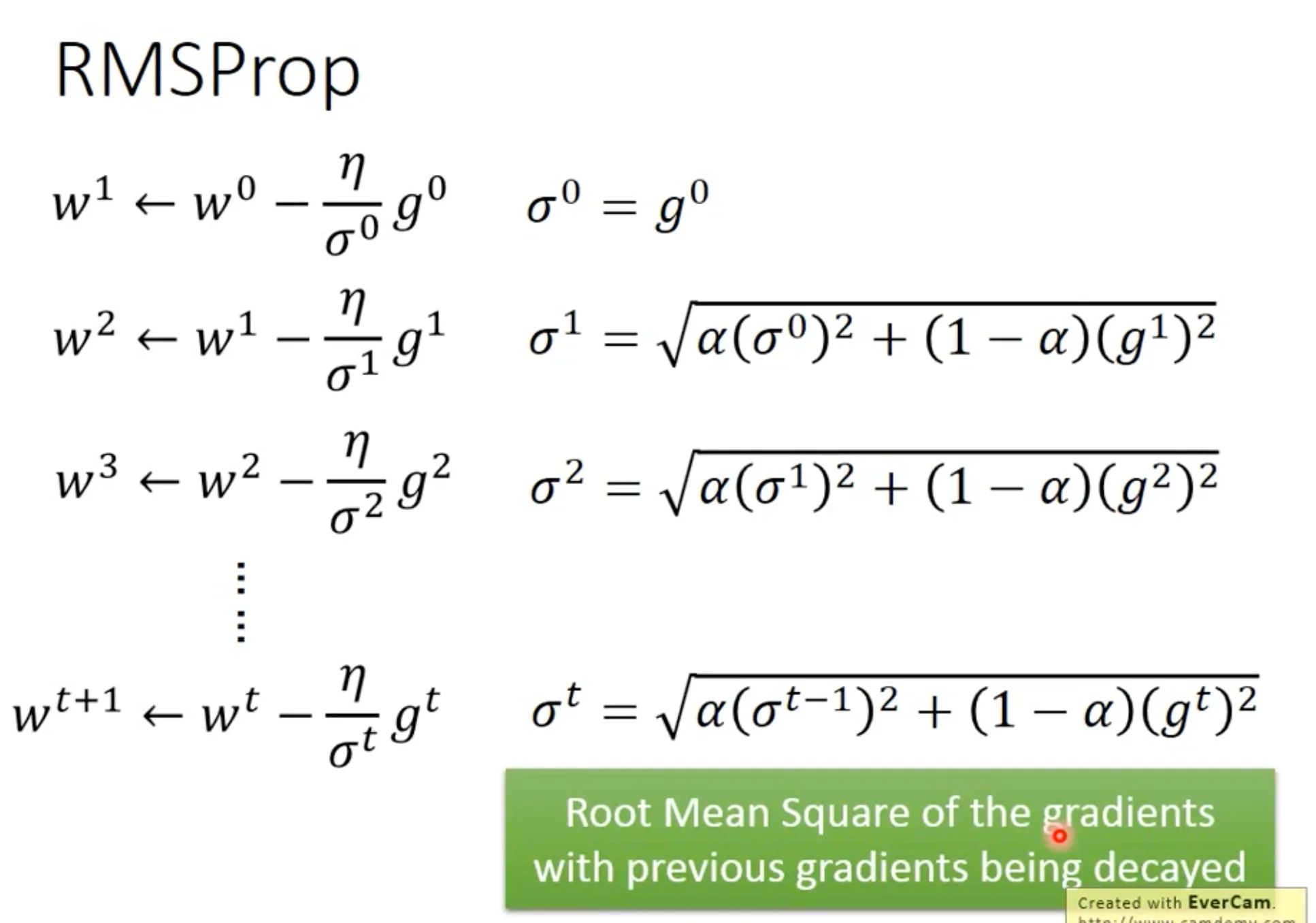
Adagrad在covex的时候效果比较好, 但是如果error surface比较复杂, 它不能很迅速地对当前地形作出反应. 于是出现了RMSProp, 更早的gradients会慢慢decay.

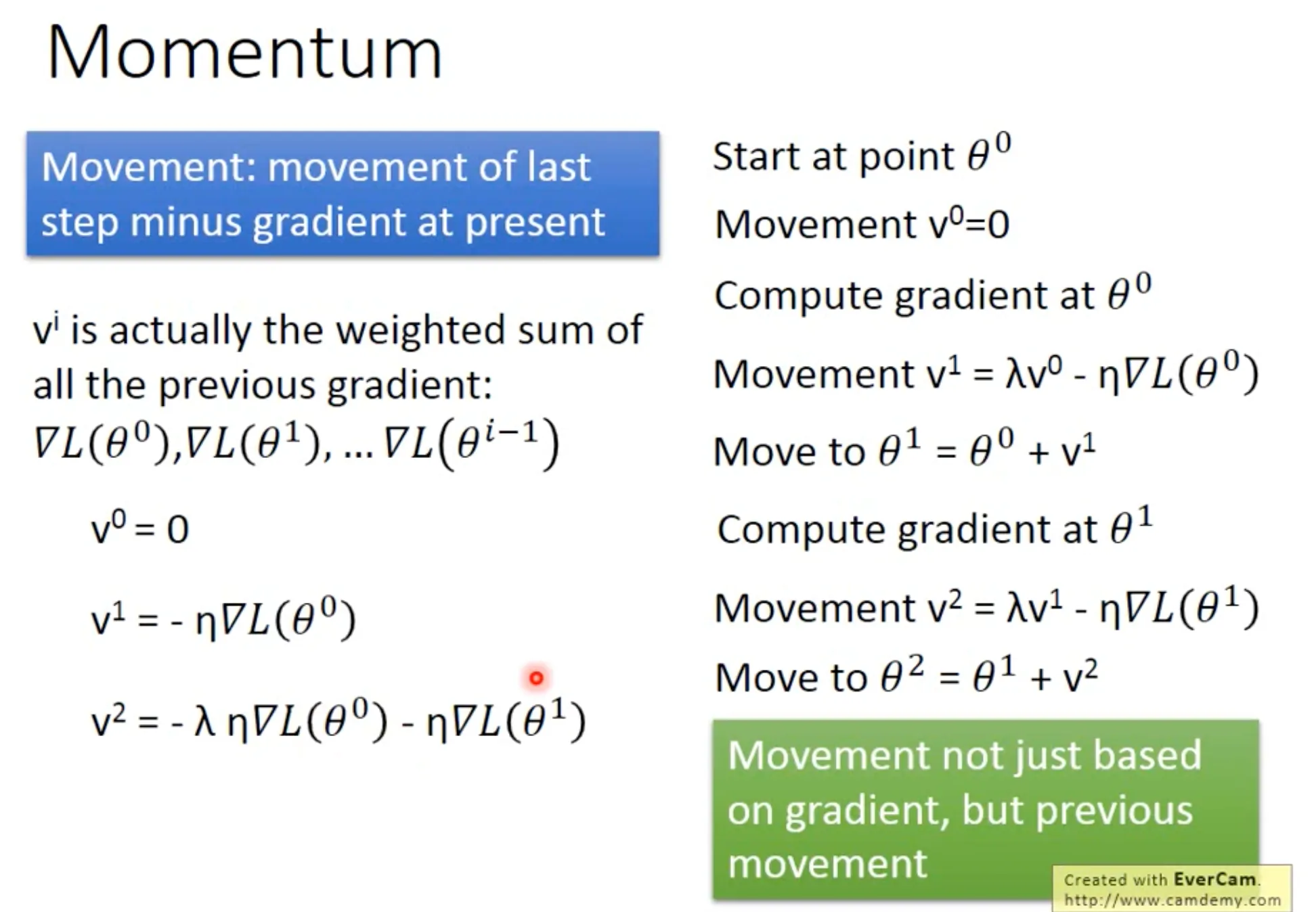
Momentum跟动量很相似, 它可以帮我们利用惯性, 跳出local minima.

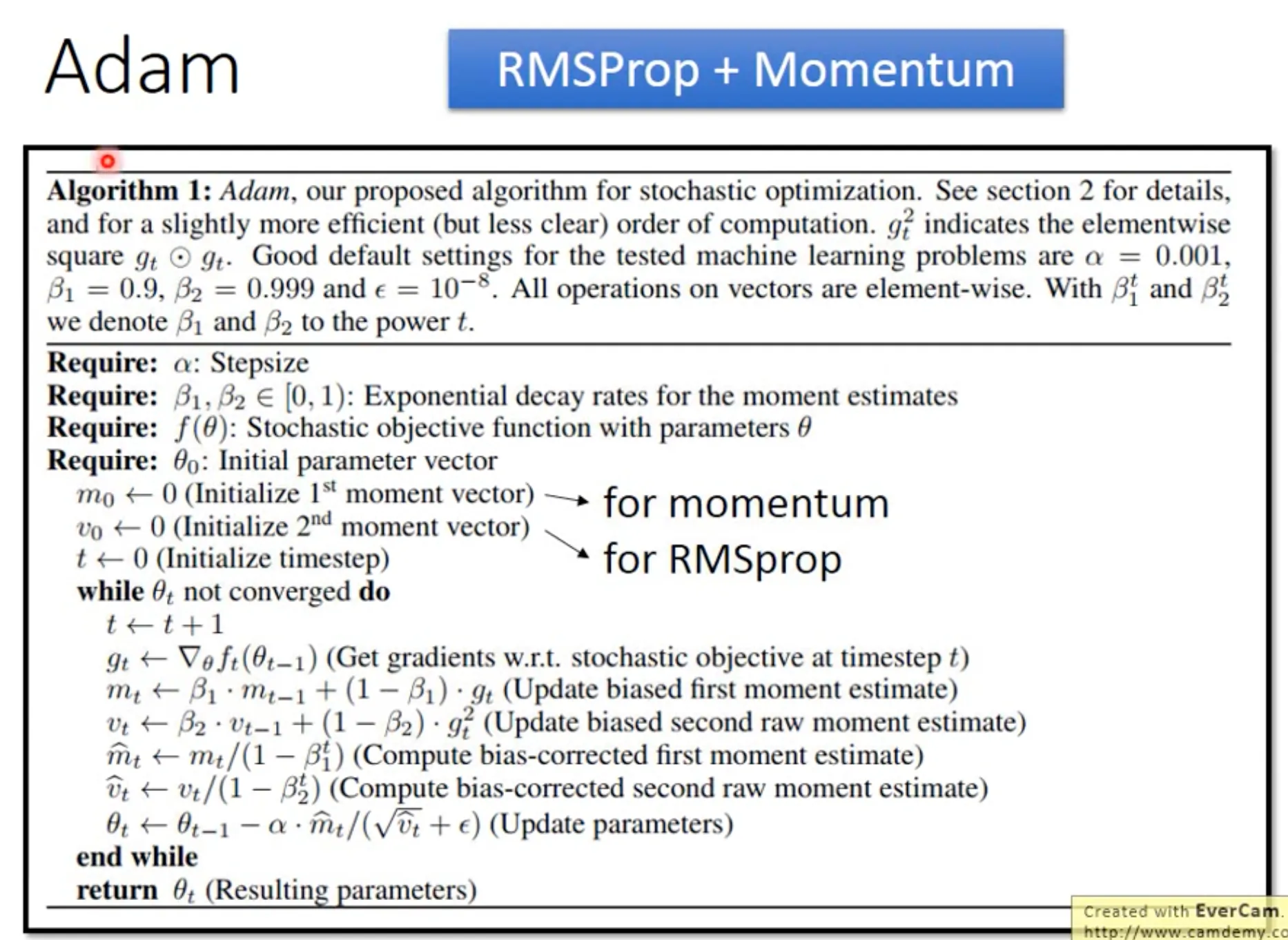
Adam可以理解为RMSProp加上Momentum (外加一个bias correction).

Improve prediction

为了避免模型overfit, 让模型更加可以推广.

• 第一个是考虑early stopping.

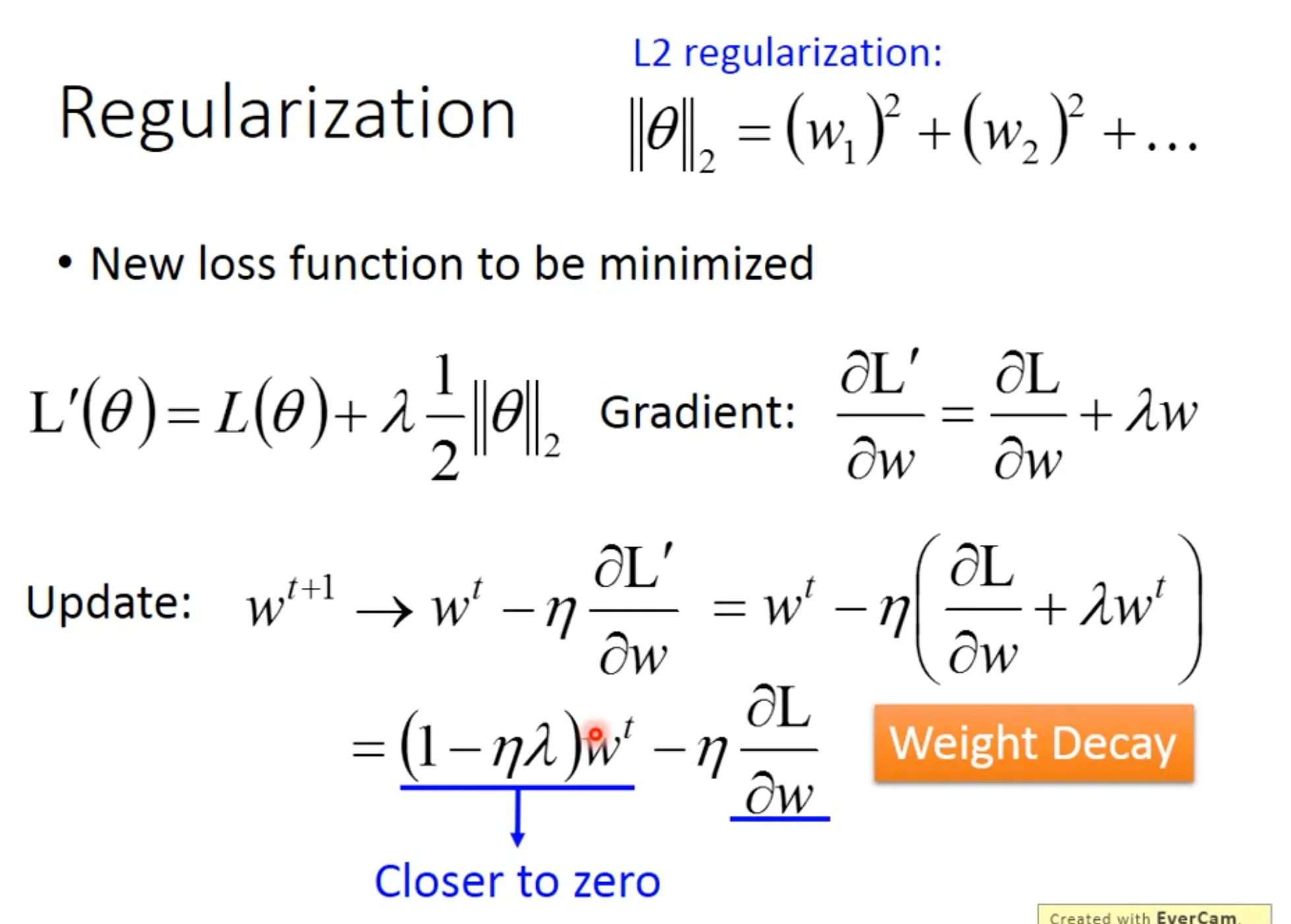
• 第二个是考虑regularization, 让$w$尽可能地小, therefore insensitive to noise. 常用L2 regularization, 可以理解为每次update的时候给$w$乘上一个$0.99$. 如果你用L1 norm来做regularization, 就相当于你每次update减去一个小的数值, 这个在你的参数很大的时候, 就没有什么效果. Regularization在SVM里面是强制的.

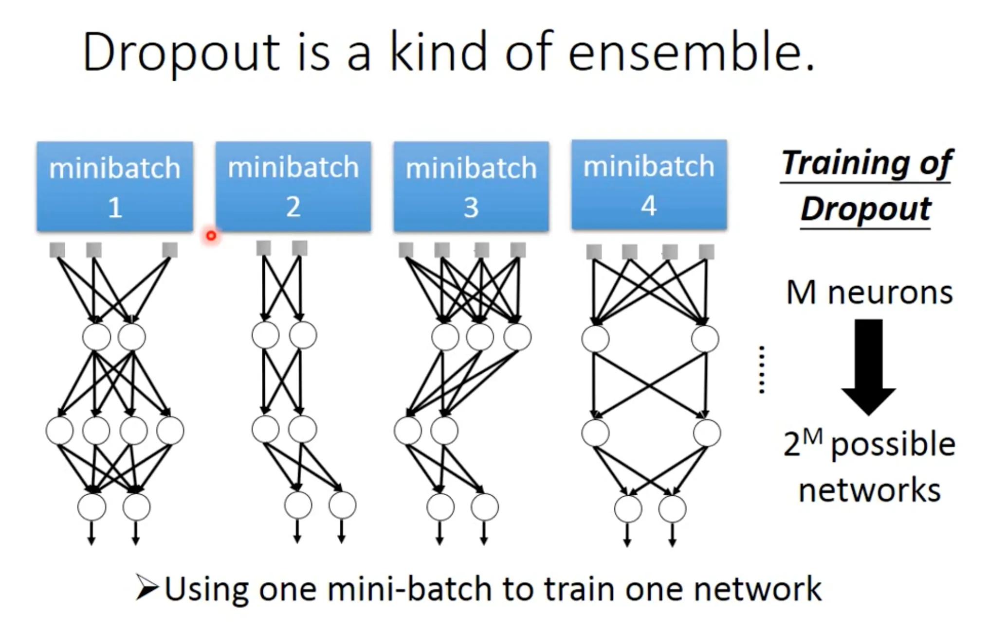
• 第三个技巧是Dropout, 这是一个神经网络特色的技巧. 记得在predict的时候adjust回你的dropout rate, 即每个参数乘上$1-p$. Dropout可以理解成一种终极的ensemble.

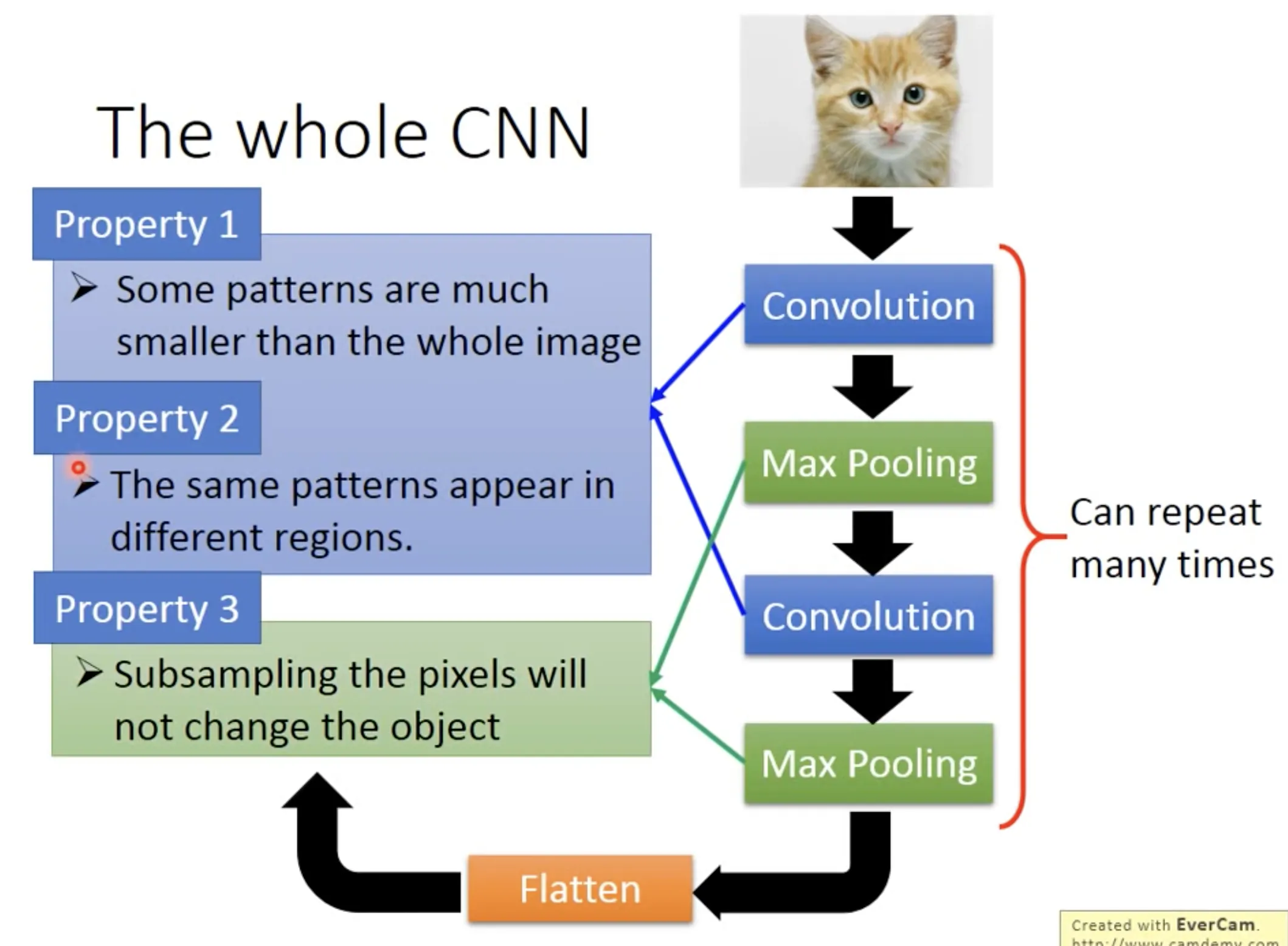
10. Convolutional Neural Network

CNN在fully connected neural network前面加入了convolution和max pooling的步骤, 主要功能是: 1.识别个别位置的特征; 2. 识别不同位置的相同特征; 3. subsample.

在Alpha Go里面, 没用max pooling, 因为显然对棋谱是不应该subsample的.

11. why Deep?