
Course notes: Infectious Disease Modelling (Imperial College London via Coursera)
Last modified:This post records the notes when I learnt the Infectious Disease Modelling (IDM) by Nimalan Arinaminpathy.
![]()
Developing the SIR Model
Backgrounds
Solving differential equations using ode() in R
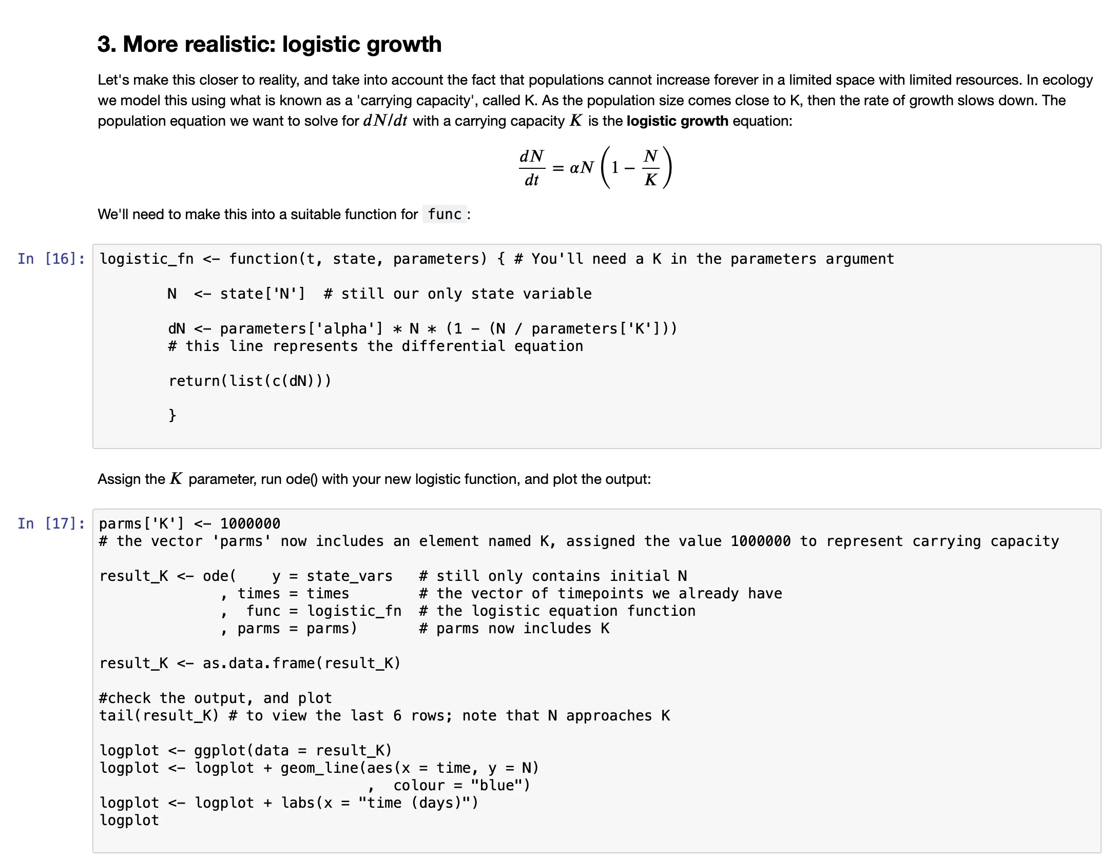
- For a quick introduction to exponential and logistic equations for population growth, visit: https://www.nature.com/scitable/knowledge/library/how-populations-grow-the-exponential-and-logistic-13240157
- For more detailed references on the deSolve package, try searching for deSolve vignettes https://cran.r-project.org/web/packages/deSolve/vignettes/deSolve.pdf
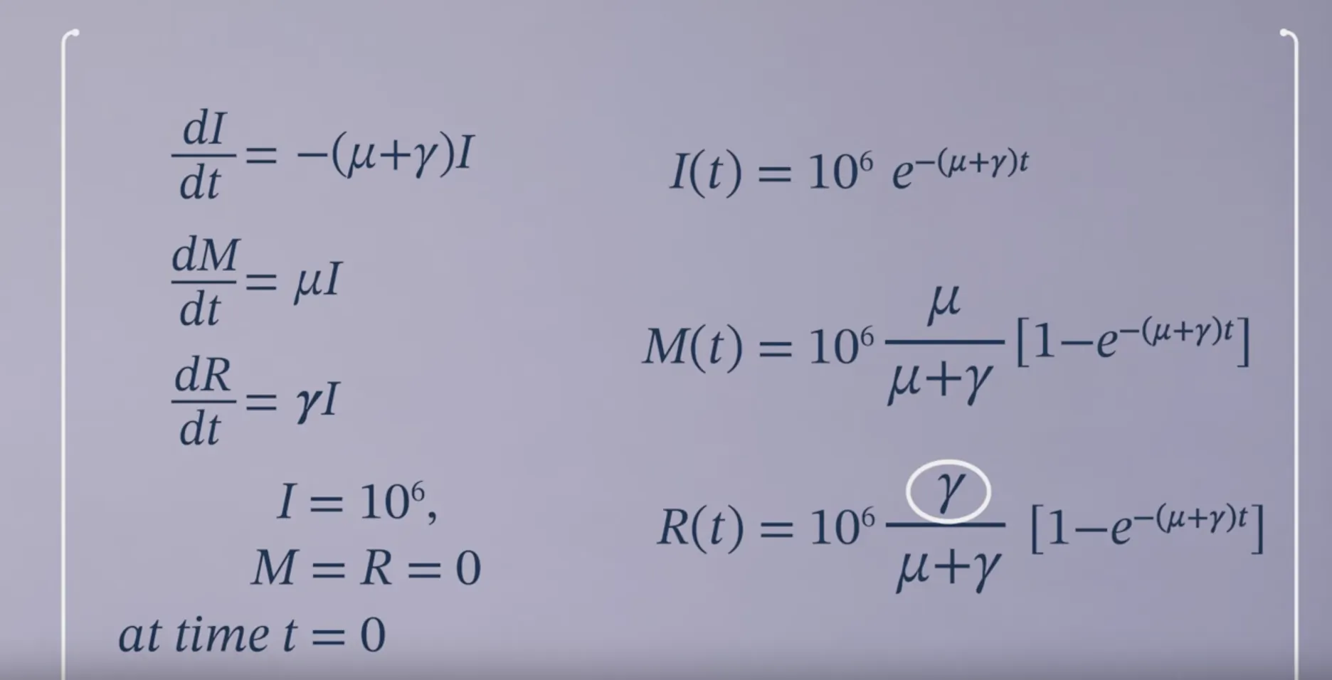
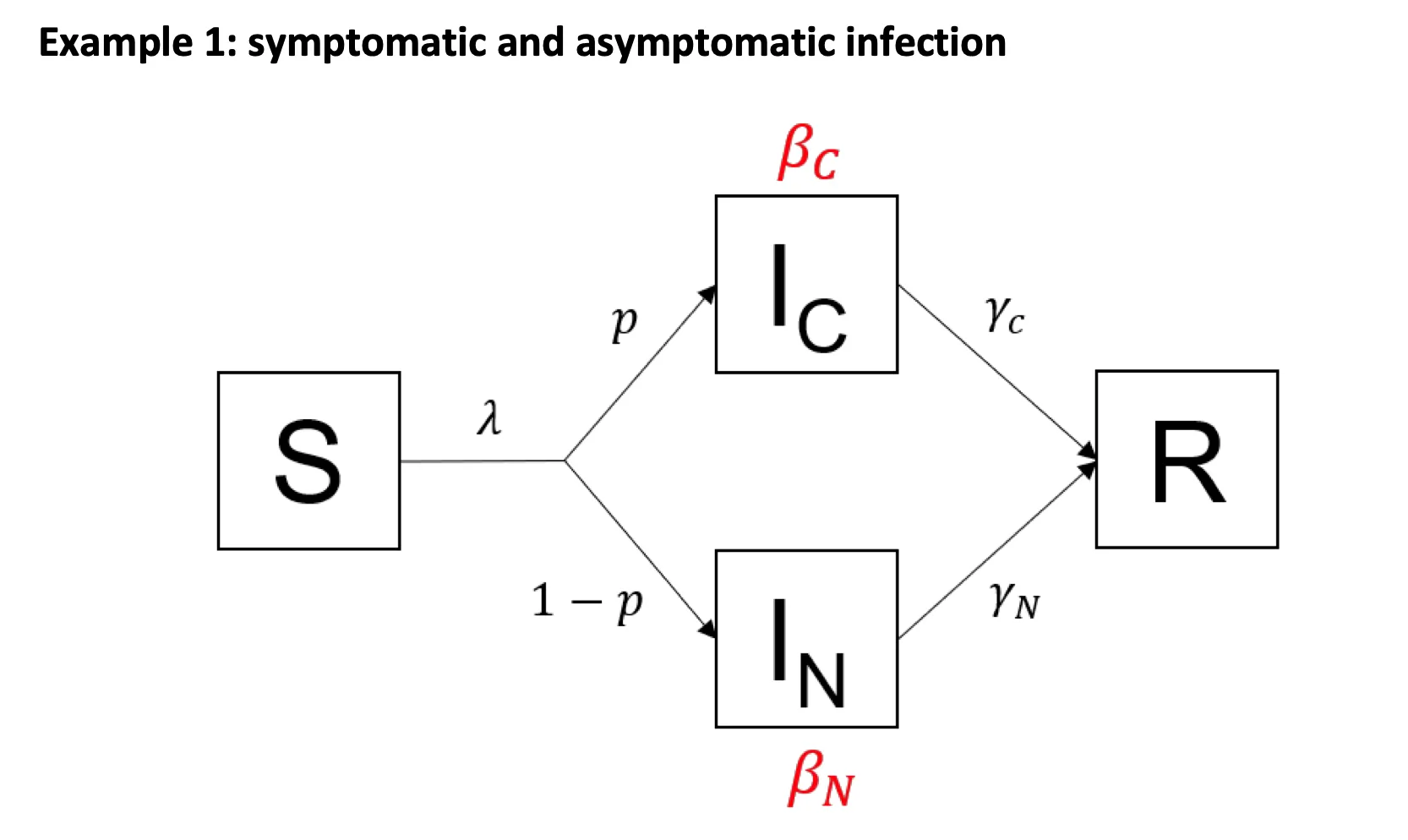
Competing Hazards in Compartmental Models
Basically $\frac{a}{a+b+c}$:
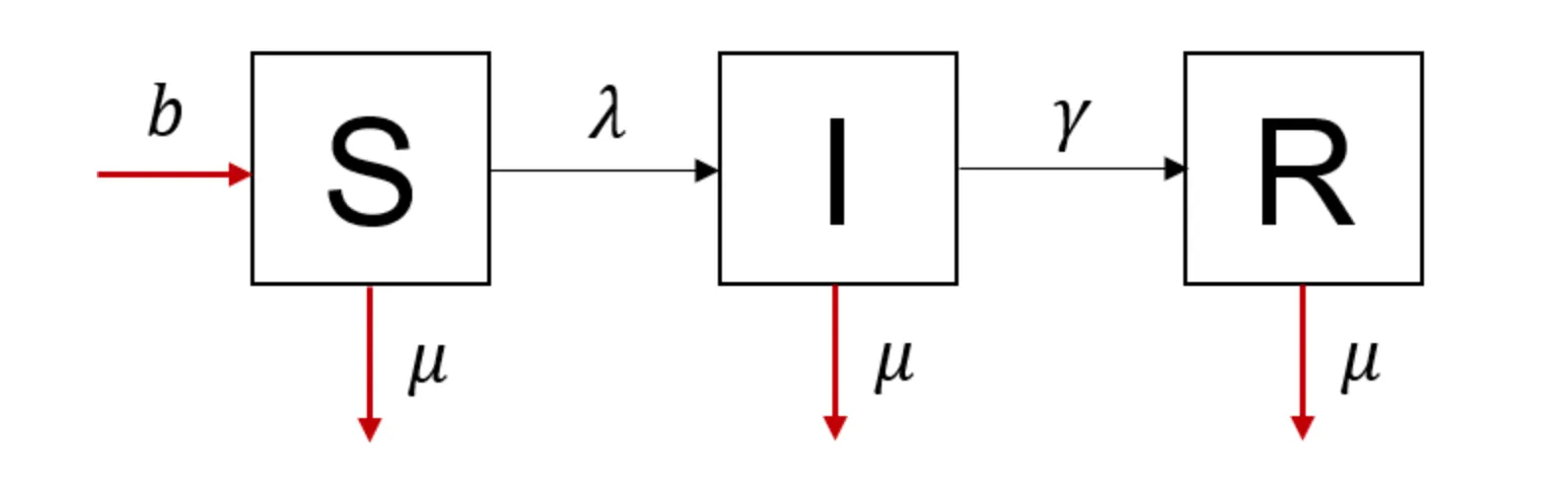
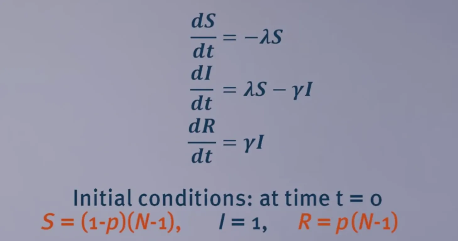
SIR Model with a Constant Force of Infection
$\lambda$: force of infection
SIR Model with a Dynamic Force of Infection
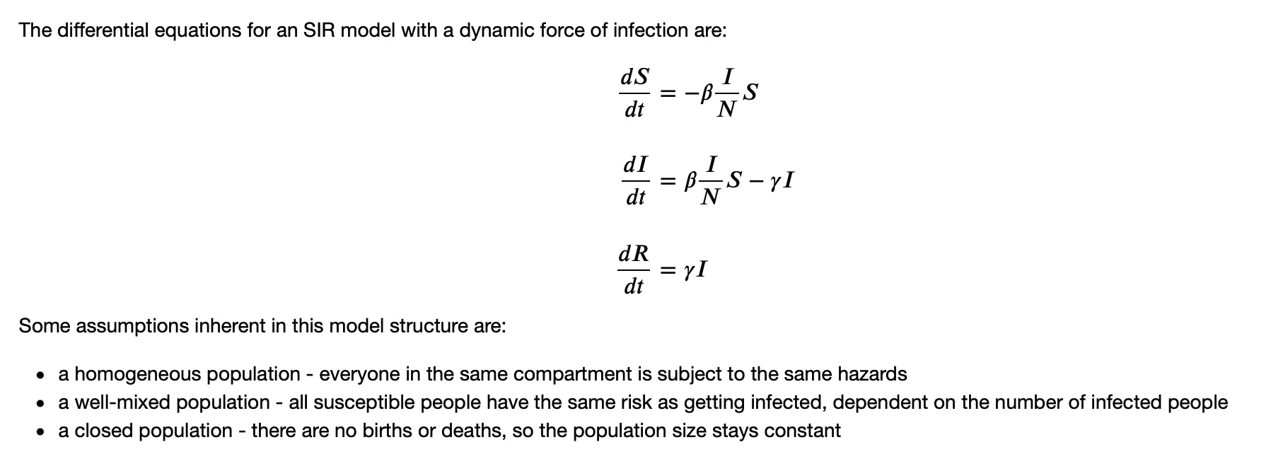
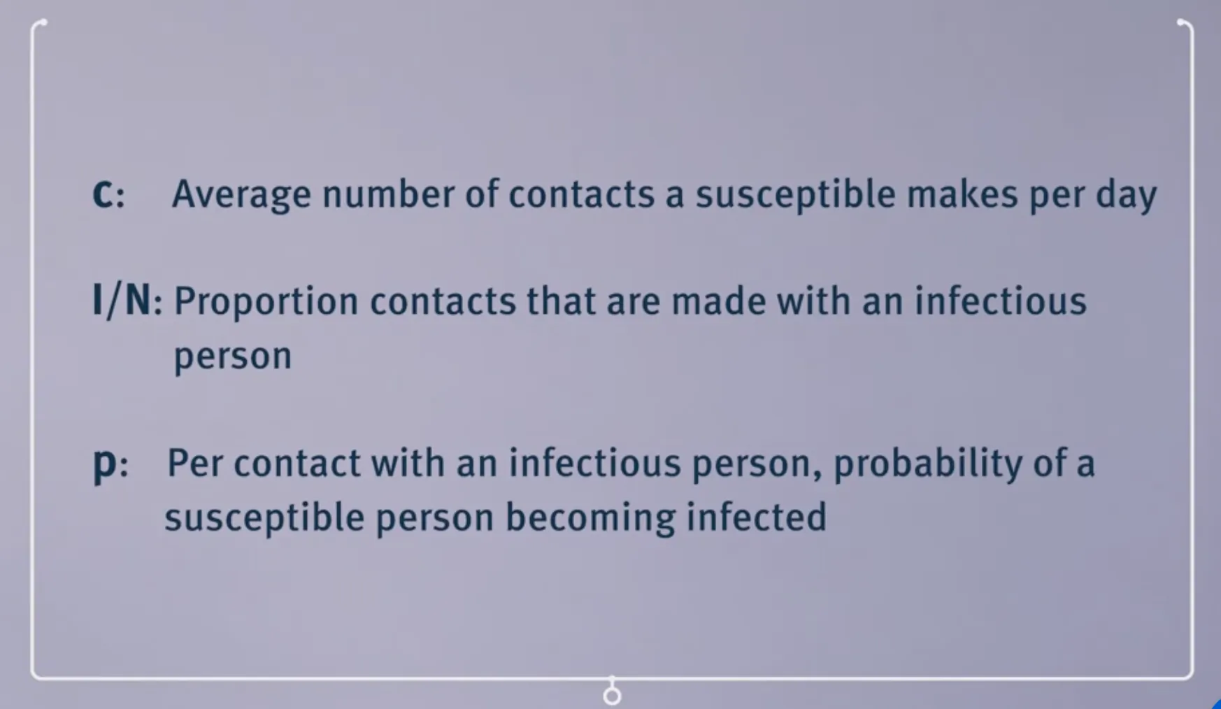
$\lambda = \beta\frac{I}{N}$ $\beta$ is the infection rate, which may be represented as $p \times c$, where $p$ is the chance of getting infection per contact, and $c$ is the number of contacts made per day.
There is a good post on difference between Density-dependent and Frequency-dependent Disease Transmission ($\beta\frac{I}{N}$ and $\beta{I}$).
# LOAD THE PACKAGES:

library(deSolve)
library(reshape2)
library(ggplot2)

# MODEL INPUTS:

initial_state_values <- c(S = 10^6-1, I = 1, R = 0)

parameters <- c(beta=1,
                gamma = 0.1)


# TIMESTEPS:

times <- seq(from = 0, to = 60, by = 1)

# SIR MODEL FUNCTION
# We are renaming this to sir_model.
# Remember to include the input arguments,
# differential equations and output objects here.

sir_model <- function(time, state, parameters) {

    with(as.list(c(state, parameters)), {
      N <- S+I+R
      lambda <- beta * (I/(N))
    # The differential equations
      dS <- -lambda * S
      dI <- -gamma * I + lambda * S
      dR <- gamma * I

    return(list(c(dS, dI, dR)))
    })

}

# MODEL OUTPUT (solving the differential equations):

output <- as.data.frame(ode(y = initial_state_values,
                            times = times,
                            func = sir_model,
                            parms = parameters))

# Plot:

output_long <- melt(as.data.frame(output), id = "time")

ggplot(data = output_long,   # specify object containing data to plot
       aes(x = time,
           y = value,
           colour = variable,
           group = variable)) +       # assign columns to axes and groups
  geom_line() +                       # represent data as lines
  xlab("Time (days)")+                # add label for x axis
  ylab("Number of people") +          # add label for y axis
  labs(colour = "Compartment")        # add legend title
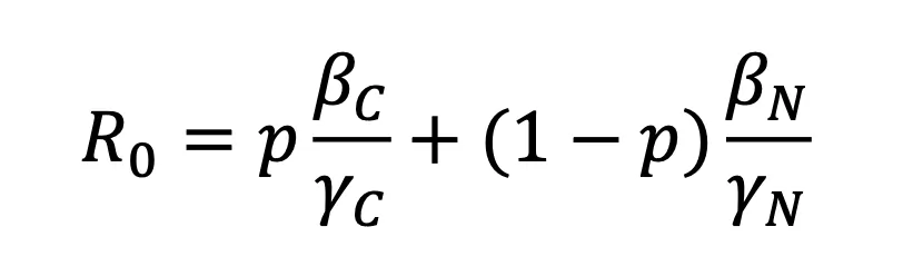
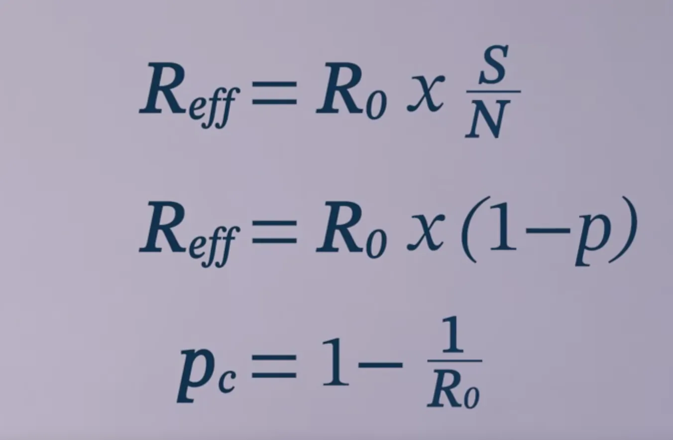
$R_0$ and $R_{eff}$
$R_0=\frac{\beta}{\gamma}$ $R_{eff} = R_0\frac{S}{N}$
Modifiers of Population Susceptibility
Modeling population turnover
A simple model for vaccination
In this simple model, $p$ of the population is immunized.
The critical vaccination threshold $p_c$ would be:
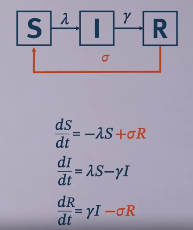
Modelling wanning immunity
Interventions and Calibration
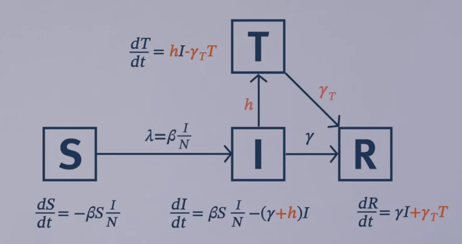
Treatment and Vaccination
Modelling treatment
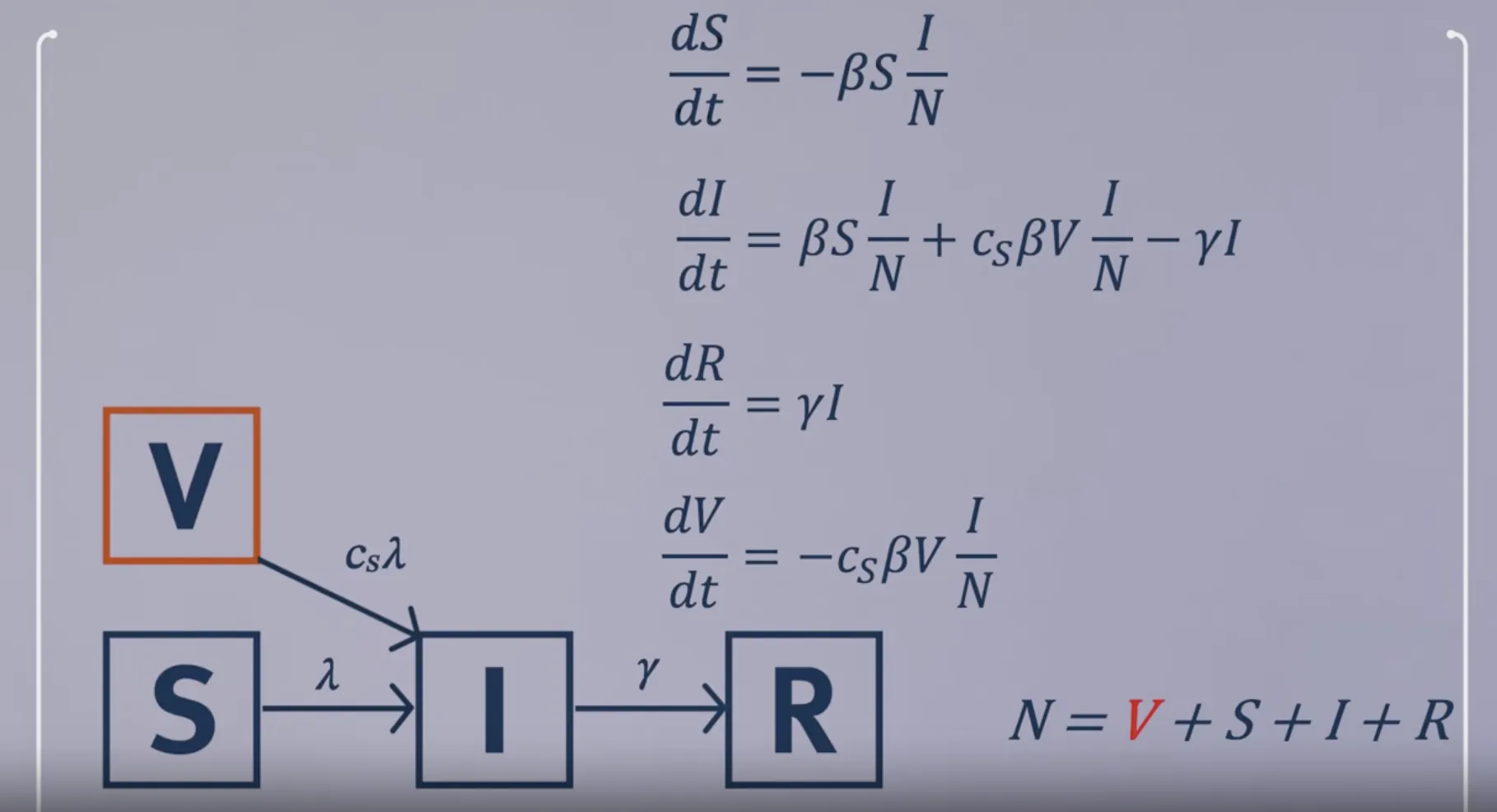
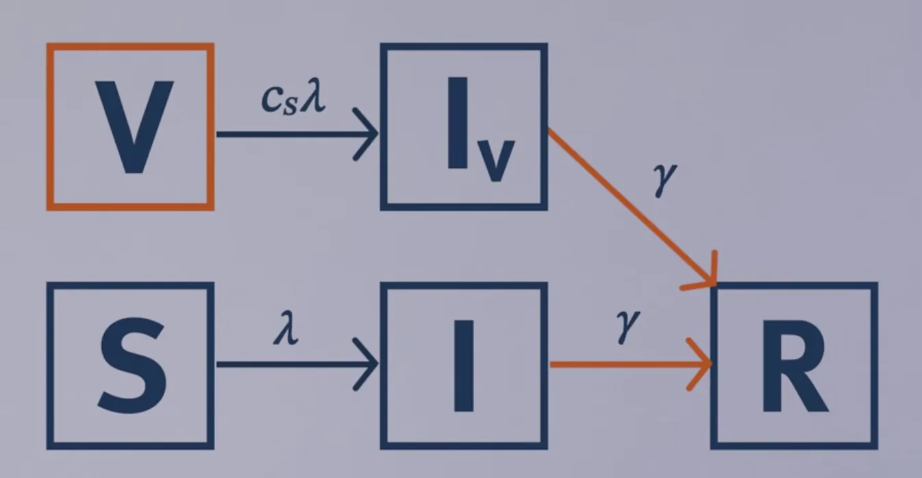
Modelling leaky vaccination
-
Vaccine reduces susceptibility $R_eff=(1-p)\times R_0 + p \times c_s\times R_0$
-
Vaccine reduces susceptibility and infectivity $R_eff = (1-p)\times \frac{\beta}{\gamma} + p \times c_s\times \frac{c_i\times \beta}{\gamma}$ $R_eff = (1-p)\times R_0 + p \times c_s\times c_i \times R_0$

# LOAD THE PACKAGES:
library(deSolve)
library(reshape2)
library(ggplot2)

# MODEL INPUTS:

# Specify the total population size
N <- 1000000

# Specify the vaccination coverage
p <- 0.6                                    # 60% coverage

# Initial number of people in each compartment
initial_state_values <- c(S = (1-p)*N,  # the unvaccinated proportion of the
                                        # population is susceptible
                          I = 1,        # the epidemic starts with a single
                                        # infected person
                          R = 0,        # there is no prior immunity in
                                        # the population
                          V = p*N,      # a proportion p of the population is
                                        # vaccinated (vaccination coverage)
                          Iv = 0)       # no vaccinated individual has been
                                        # infected at the beginning of the
                                        # simulation

# Parameters
parameters <- c(beta = 0.25,     # the infection rate in units of days^-1
                gamma = 0.1,     # the rate of recovery in units of days^-1
                c_s = 0.3,       # the reduction in the force of infection
                                # acting on those vaccinated
                c_i = 0.5)       # the reduction in the infectivity of
                                # vaccinated infected people

# TIMESTEPS:

# Sequence of timesteps to solve the model at
times <- seq(from = 0, to = 730, by = 1)   # from 0 to 2 years, daily intervals

# MODEL FUNCTION:

vaccine_model <- function(time, state, parameters) {

    with(as.list(c(state, parameters)), {

    # Defining lambda as a function of beta and I:
      lambda <- beta * I/N + c_i * beta * Iv/N
    # the Iv compartment is c_i times less infectious than the I compartment

    # The differential equations
      dS <- -lambda * S
      dI <- lambda * S - gamma * I
      dR <- gamma * I + gamma * Iv            # infected and vaccinated infected
                                              # individuals recover at the same rate
      dV <- -c_s * lambda * V                 # vaccinated people become infected at
                                              # a rate c_s * lambda
      dIv <- c_s * lambda * V - gamma * Iv    # vaccinated people who become infected
                                              # move into the Iv compartment

    # Return the number of people in each compartment at each timestep
    # (in the same order as the input state variables)
    return(list(c(dS, dI, dR, dV, dIv)))
    })

}

# MODEL OUTPUT:

# Solving the differential equations using the ode integration algorithm
output <- as.data.frame(ode(y = initial_state_values,
                            times = times,
                            func = vaccine_model,
                            parms = parameters))

# PLOT THE OUTPUT

# Plot the number of infected people over time
ggplot(data = output,
      aes(x = time, y = I+Iv)) +   # infected people are in the I and Iv compartment
  geom_line() +
  xlab("Time (days)")+
  ylab("Number of infected people") +
  labs(title = paste("Combined leaky vaccine with coverage of", p*100, "%"))
Calibration
Automated Least-Squares Calibration
require(deSolve)

SIR_fn <- function(time, state, parameters) {

    with(as.list(c(state, parameters)), {
        N  <- S+I+R

        dS <- -beta*S*I/N
        dI <- beta*S*I/N-gamma*I
        dR <- gamma*I

        return(list(c(dS, dI, dR)))

    })

}

SIR_SSQ <- function(parameters, dat) {  # parameters must contain beta & gamma

    # calculate model output using your SIR function with ode()

    result <- as.data.frame(ode(y = initial_state_values  # vector of initial state
                                                          # values, with named elements
                              , times = times             # vector of times
                              , func = SIR_fn             # your predefined SIR function
                              , parms = parameters)       # the parameters argument
                                                          # entered with SIR_SSQ()
    )

    # SSQ calculation: needs the dat argument (the observed data you are fitting to)
    # assumes the data you are fitting to has a column "I"

    # select only complete cases, i.e. rows with no NAs, from the dataframe
    dat <- na.omit(dat)

    # select elements where results$time is in dat$time
    deltas2 <- (result$I[result$time %in% dat$time]
                - dat$I)^2
    SSQ   <- sum(deltas2)

    return(SSQ)

    }
flu_dat <- data.frame(time = c(1:14),
                      I = c(3, 8, 26, 76, 225, 298, 258, 233, 189, 128, 68, 29, 14, 4))

initial_state_values <- c(S = 762, I = 1, R = 0)

# choose values to start your optimisation
beta_start  <- 1
gamma_start <- 0.5

# times - dense timesteps for a more detailed solution
times <- seq(from = 0, to = 14, by = 0.1)

# optim
# you will need to run the cells to assign your functions first

optimised <- optim(par = c(beta = beta_start
                        , gamma = gamma_start)      # these are the starting beta
                                                    # and gamma that will be fed
                                                    # first, into SSQ_fn
                        , fn = SIR_SSQ
                        , dat = flu_dat  # this argument comes under "..."
                                         # "Further arguments to be passed to fn and gr"
      )

optimised #have a look at the model output
optimised$par

opt_mod <- as.data.frame(ode(y = initial_state_values  # named vector of initial
                                                       # state values
                            , times = times            # vector of times
                            ,  func = SIR_fn           # your predefined SIR function
                            , parms = optimised$par))
## plot your optimised model output, with the epidemic data using ggplot ##
require(ggplot2)

opt_plot <- ggplot()
opt_plot <- opt_plot + geom_point(aes(x = time, y = I)
                                , colour = "red"
                                , shape  = "x"
                                , data = flu_dat)
opt_plot <- opt_plot + geom_line(aes(x = time, y = I)
                                 , colour = "blue"
                                 , data   = opt_mod)
opt_plot
Likelihoods
# Load the flu dataset of reported cases
reported_data <- read.csv("../Graphics_and_Data/idm2_sir_reported_data.csv")

# PACKAGES
require(deSolve)
require(ggplot2)

# INPUT
initial_state_values <- c(S = 762,
                          I = 1,
                          R = 0)

times <- seq(from = 0, to = 14, by = 0.1)

# SIR MODEL FUNCTION
sir_model <- function(time, state, parameters) {

  with(as.list(c(state, parameters)), {

    N <- S+I+R

    lambda <- beta * I/N

    # The differential equations
    dS <- -lambda * S
    dI <- lambda * S - gamma * I
    dR <- gamma * I

    # Output
    return(list(c(dS, dI, dR)))
  })
}

# DISTANCE FUNCTION

loglik_function <- function(parameters, dat) {   # takes as inputs the parameter values and dataset

   beta <- parameters[1]    # extract and save the first value in the "parameters" input argument as beta
   gamma <- parameters[2]   # extract and save the second value in the "parameters" input argument as gamma

   # Simulate the model with initial conditions and timesteps defined above, and parameter values from function call
   output <- as.data.frame(ode(y = initial_state_values,
                               times = times,
                               func = sir_model,
                               parms = c(beta = beta,       # ode() takes the values for beta and gamma extracted from
                                         gamma = gamma)))   # the "parameters" input argument of the loglik_function()

   # Calculate log-likelihood using code block 4 from the previous etivity, accounting for the reporting rate of 60%:
   LL <- sum(dpois(x = dat$number_reported, lambda = 0.6 * output$I[output$time %in% dat$time], log = TRUE))

   return(LL)
}

# OPTIMISATION

optim(par = c(1.7, 0.1),           # starting values for beta and gamma - you should get the same result no matter
                                   # which values you choose here
      fn = loglik_function,        # the distance function to optimise
      dat = reported_data,         # the dataset to fit to ("dat" argument is passed to the function specified in fn)
      control = list(fnscale=-1))  # tells optim() to look for the maximum number instead of the minimum (the default)
Building on the SIR Model
Stochastic and Deterministic Models
All the above models are Deterministic Models. We could use Gillespie algorithm to model stochastic SIR model.
Age-structured model
We can apply contact matrix as a parameter to model the transmission between different age groups.
# INPUT
# Initial state values for a naive population (everyone is susceptible except for 1 index case),
# where the total population size N is (approximately) 1 million, 20% of this are children and 15% are elderly
initial_state_values <- c(S1 = 200000,   # 20% of the population are children - all susceptible
                          S2 = 650000,   # 100%-20%-15% of the population are adults - all susceptible
                          S3 = 150000,   # 15% of the population are elderly - all susceptible
                          I1 = 1,        # the outbreak starts with 1 infected person (can be of either age)
                          I2 = 0,
                          I3 = 0,
                          R1 = 0,
                          R2 = 0,
                          R3 = 0)

# Set up an empty contact matrix with rows for each age group and columns for each age group
contact_matrix <- matrix(0,nrow=3,ncol=3)
# Fill in the contract matrix
contact_matrix[1,1] = 7     # daily number of contacts that children make with each other
contact_matrix[1,2] = 5     # daily number of contacts that children make with adults
contact_matrix[1,3] = 1     # daily number of contacts that children make with the elderly
contact_matrix[2,1] = 2     # daily number of contacts that adults make with children
contact_matrix[2,2] = 9     # daily number of contacts that adults make with each other
contact_matrix[2,3] = 1     # daily number of contacts that adults make with the elderly
contact_matrix[3,1] = 1     # daily number of contacts that elderly people make with children
contact_matrix[3,2] = 3     # daily number of contacts that elderly people make with adults
contact_matrix[3,3] = 2     # daily number of contacts that elderly people make with each other
# The contact_matrix now looks exactly like the one in the etivity instructions. We add this matrix as a parameter below.

# Parameters
parameters <- c(b = 0.05,     # the probability of infection per contact is 5%
                contact_matrix = contact_matrix,   # the age-specific average number of daily contacts (defined above)
                gamma = 1/5)  # the rate of recovery is 1/5 per day

# Run simulation for 3 months
times <- seq(from = 0, to = 90, by = 0.1)

# MODEL FUNCTION
sir_age_model <- function(time, state, parameters) {

  with(as.list(parameters), {

    n_agegroups <- 3                                 # number of age groups
    S <- state[1:n_agegroups]                        # assign to S the first 3 numbers in the initial_state_values vector
    I <- state[(n_agegroups+1):(2*n_agegroups)]      # assign to I numbers 4 to 6 in the initial_state_values vector
    R <- state[(2*n_agegroups+1):(3*n_agegroups)]    # assign to R numbers 7 to 9 in the initial_state_values vector

    N <- S+I+R     # people in S, I and R are added separately by age group, so N is also a vector of length 3

    # Defining the force of infection

    # Force of infection acting on susceptible children
    lambda <- b * contact_matrix %*% as.matrix(I/N)
    # %*% is used to multiply matrices in R
    # the lambda vector contains the forces of infection for children, adults and the elderly (length 3)

    # The differential equations
    # Rate of change in children:
    dS <- -lambda * S
    dI <- lambda * S - gamma * I
    dR <- gamma * I

    # Output
    return(list(c(dS, dI, dR)))
  })
}


# MODEL OUTPUT

output <- as.data.frame(ode(y = initial_state_values,
                            times = times,
                            func = sir_age_model,
                            parms = parameters))
# the output column names are adopted from the names we assigned in the initial_state_values vector

# Turn output into long format
output_long <- melt(as.data.frame(output), id = "time")

# Plot number of people in all compartments over time
ggplot(data = output_long,
       aes(x = time, y = value, colour = variable, group = variable)) +
  geom_line() +
  xlab("Time (days)")+
  ylab("Number of people") +
  labs(colour = "Compartment")
Modelling Vector-Borne Diseases
The structure of a VBD model is shown below:
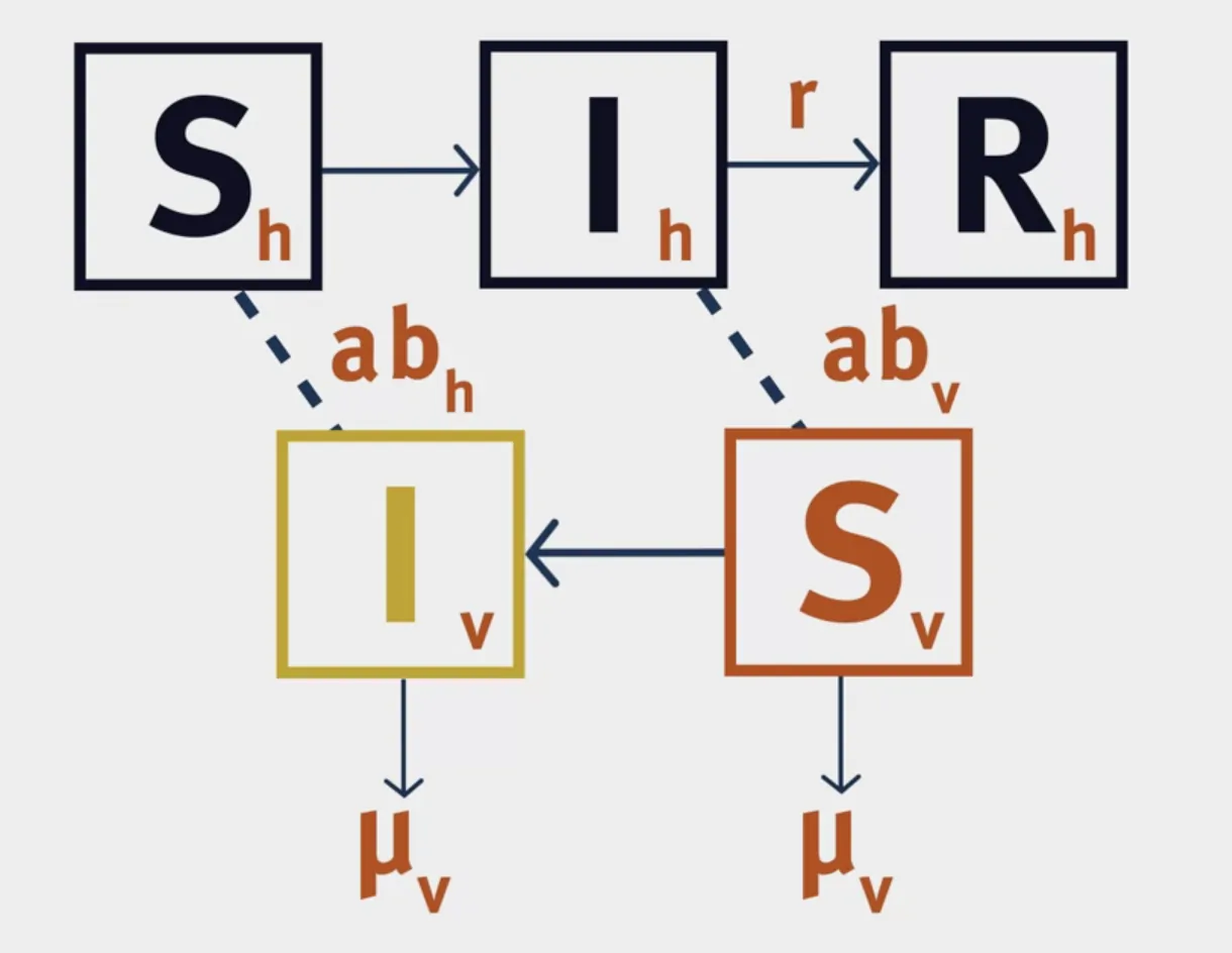 $a$ is the biting rate of mosquitoes.
$b$ is the probability of infection following a bite.
$a$ is the biting rate of mosquitoes.
$b$ is the probability of infection following a bite.


Vectorial Capacity: The number of secondary cases arising per day from a single infected case in a totally susceptible human population.
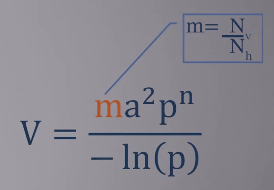
- What is $p^n$? $p$ is the probability of the vector surviving through one day and $n$ is the average duration of the extrinsic incubation period in days, so $p^n$ is the probability of the vector surviving through the extrinsic incubation period.
# INPUT
Nh <- 10000   # total number of hosts
Nv <- 20000   # total number of vectors

initial_state_values <- c(Sh = Nh-0.0028*Nh,
                          Ih = 0.0028*Nh,
                          Rh = 0,
                          Sv = Nv-0.00057*Nv,
                          Iv = 0.00057*Nv)

parameters <- c(a = 1,       # mosquito biting rate per day
                b_v = 0.4,   # probability of infection from an infected host to a susceptible vector
                b_h = 0.4,   # probability of infection from an infected vector to a susceptible host
                u_v = 0.25,  # mortality/recruitment rate of the vector
                r = 0.167)   # recovery rate from dengue in humans

times <- seq(from = 0, to = 90, by = 1)    # simulate for 3 months (90 days)

# SIR MODEL FUNCTION
vbd_model <- function(time, state, parameters) {

  with(as.list(c(state, parameters)), {

    Nh <- Sh + Ih + Rh   # total human population
    Nv <- Sv + Iv        # total vector population

    # The differential equations
    # Host population dynamics:
    dSh <- -a*b_h*Sh*Iv/Nh
    dIh <- a*b_h*Sh*Iv/Nh - r * Ih
    dRh <- r * Ih
    # Vector population dynamics:
    dSv <- u_v * Nv - a*b_v*Sv*Ih/Nh - u_v * Sv
    dIv <- a*b_v*Sv*Ih/Nh - u_v * Iv

    # Output
    return(list(c(dSh, dIh, dRh, dSv, dIv)))
  })
}
Next
Study the partially observed Markov process (POMP) models and package.
Tags: Infectious disease modelling
Categories: Course notes
Comments