Paper digest: Informing policy via dynamic models: cholera in Haiti (Jesse Wheeler)

This paper is from Edward L. Ionides et al. It considers the 2010-2019 cholera epidemic in Haiti, and studies three dynamic models developed by expert teams to advise on vaccination policies. Importantly, the paper demonstrates the basic usage of the SpatPOMP model. The code and software are also provided.

Introduction

Population dynamics may be nonlinear and stochastic, with the resulting complexities compounded by incomplete understanding of the underlying biological mechanisms and by partial observability of the system variables. Quantitative models for these dynamic systems offer potential for designing effective control measures.

Questions of interest include:

• What indications should we look for in the data to assess whether the model-based inferences are trustworthy?
• What diagnostic tests and model variations can and should be considered in the course of the data analysis?
• What are the possible trade-offs of increasing model complexity, such as the inclusion of interactions across spatial units?

Three models from different expert groups were considered:

• Model 1 is stochastic and describes cholera at the national level;
• Model 2 is deterministic with spatial structure, and includes transmission via contaminated water;
• Model 3 is stochastic with spatial structure, and accounts for measured rainfall.

The groups largely adhered to existing guidelines on creating models to inform policy (Behrend et al., 2020; Saltelli et al., 2020)

Mechanistic models for cholera in Haiti

• Models that focus on learning relationships between variables in a dataset are called associative, whereas models that incorporate a known scientific property of the system are called causal or mechanistic.
• Lucas critique: Lucas et al. (1976) pointed out that it is naive to predict the effects of an intervention on a given system based entirely on historical associations.
• Model 1: The model was implemented by a team at Johns Hopkins Bloomberg School of Public Health (here- after referred to as the Model 1 authors) in the R programming language using the pomp package (King et al., 2016). Original source code is publicly available with DOI: 10.5281/zenodo.3360991.
  • SEIAR model: describes susceptible, latent (exposed), infected (and symptomatic), asymptomatic, and recovered individuals in vaccine cohort $z$. Here, $z = 0$ corresponds to unvaccinated individuals, and $z ∈ 1:Z$ describes hypothetical vaccination programs.
  • Reported cholera cases at time point $n$ ($Y_n$) are assumed to come from a negative binomial measurement model, where only a fraction ($ρ$) of new weekly cases are reported.
• Model 2: Model 2 was developed by a team that consisted of members from the Fred Hutchinson Cancer Research Center and the University of Florida (hereafter referred to as the Model 2 authors). While Model 2 is the only deterministic model we considered in our analysis, it contains perhaps the most complex descriptions of cholera in Haiti: Model 2 accounts for movement between spatial units; human-to-human and environment-to-human cholera infections; and transfer of water between spatial units based on elevation charts and river flows. The source code that the Model 2 authors used to generate their results was written in the Python programming language, and is publicly available at 10.5281/zenodo.3360857 and its accompanying GitHub repository https://github.com/lulelita/HaitiCholeraMultiModelingProject.
  • Susceptible individuals are in compartments $S_{uz}(t)$, where $u ∈ 1:U$ corresponds to the $U = 10$ departments, and $z ∈ 0:4$ describes vaccination status:
    • z = 0: Unvaccinated or waned vaccination protection.
    • z = 1: One dose at age under five years.
    • z = 2: Two doses at age under five years.
    • z = 3: One dose at age over five years.
    • z = 4: Two doses at age over five years.
  • Individuals can progress to a latent infection $E_{uz}$ followed by symptomatic infection $I_{uz}$ with recovery to $R_{uz}$ or asymptomatic infection $A_{uz}$ with recovery to $R^A_{uz}$. The force of infection depends on both direct transmission and an aquatic reservoir, $W_u(t)$.
  • Reported cases are assumed to come from a log-normal distribution, with the log-scale mean equal to the reporting rate $ρ$ times the number of newly infected individuals.
• Model 3: Model 3 was developed by a team of researchers at the Laboratory of the Swiss Federal Institute of Technology in Lausanne, hereafter referred to as the Model 3 authors. The code that was originally used to implement Model 3 is archived with the DOI: 10.5281/zenodo.3360723, and also available in the public GitHub repository: jcblemai/haiti-mass-ocv-campaign.
  • The latent state is described as $X(t)=(S_{uz}(t), I_{uz}(t), A_{uz}(t), R_{uzk}(t), W_{u}(t), u \in 0:U, z \in 0:4, k \in 1:3)$. $k ∈ 1:3$ models non-exponential duration in the recovered class before waning of immunity.
  • Reported cholera cases are assumed to come from a negative binomial measurement model with mean equal to a fraction ($ρ$) of individuals in each unit who develop symptoms and seek healthcare.

Statistical Analysis

Model Fitting

Each of the three models considered in this study describes cholera dynamics as a partially observed Markov process (POMP). Each model is indexed by a parameter vector, $θ$, and different values of $θ$ can result in qualitative differences in the predicted behavior of the system.

• Elements of $θ$ can be fixed at a constant value based on scientific understanding of the system, but parameters can also be calibrated to data by maximizing a measure of congruency between the observed data and the assumed mechanistic structure.
• Cali- brating model parameters to observed data does not guarantee that the resulting model successfully approximates real-world mechanisms, since model assumptions may be incorrect, and do not change as the model is calibrated to data. However, the congruency between the model and observed data serves as a proxy for the congruency between the model and the true underlying dynamic system.

Calibrating Model 1 Parameters

• In order to retain the ability to propose models that are scientifically meaningful rather than only those that are simply statistically convenient, we restrict ourselves to parameter estimation techniques that have the plug- and-play property, which is that the fitting procedure only requires the ability to simulate the latent process instead of evaluating transition densities.
• To our knowledge, the only plug-and-play, frequentist methods that can maximize the likelihood for POMP models of this complexity are iterated filtering algorithms (Ionides et al., 2015), which modify the well-known particle filter (Arulampalam et al., 2002) by performing a random walk for each parameter and particle.

Calibrating Model 2 Parameters

• Because the process model of Model 2 is deterministic, the parameter estimation problem for Model 2 reduces to a least squares calculation when combined with a Gaussian measurement model.
• The inclusion of a change-point in model states and parameters increases the flexibility of the model and hence the ability to fit the observed data. The increase in model flexibility, however, results in hidden states that are inconsistent between model phases.
• We fit the model to log-transformed case counts, since the log scale stabilizes the variation during periods of high and low incidence. An alternative solution is to change the measurement model to include overdispersion, as was done in Models 1 and 3.

Calibrating Model 3 Parameters

• Model 3 describes cholera dynamics in Haiti using a metapopulation model, where the hidden states in each administrative department has an effect on the dynamics in other departments. The decision to address metapopulation dynamics using a spatially explicit model, rather than to aggregate over space, is double-edged.
• We calibrate the parameters of the spatially coupled version of Model 3 using the iterated block particle filter (IBPF) algorithm of Ionides, Ning and Wheeler (2022).

Model Diagnostics

• Parameter calibration (whether Bayesian or frequentist) aims to find the best description of the observed data under the assumptions of the model. Obtaining the best fitting set of parameters for a given model does not, however, guarantee that the model provides an accurate representation of the system in question. Model misspecification, which may be thought of as the omission of a mechanism in the model that is an important feature of the dynamic system, is inevitable at all levels of model complexity.
• In this section, we discuss some tools for diagnosing mechanistic models with the goal of making the subjective assessment of model “usefulness” more objective. To do this, we will rely on the quantitative and statistical ability of the model to match the observed data, which we call the model’s goodness-of-fit, with the guiding principle that a model which cannot adequately describe observed data may not be reliable for useful purposes.
• One common approach to assess a mechanistic model’s goodness-of-fit is to compare simulations from the fitted model to the observed data.
• Another approach is to compare a quantitative measure of the model fit (such as MSE, predictive accuracy, or model likelihood) among all proposed models.
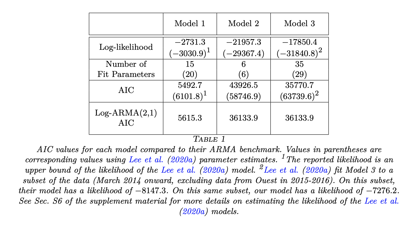
• To calibrate relative measures of fit, it is useful to compare against a model that has well-understood statistical ability to fit data, and we call this model a benchmark. Standard statistical models, interpreted as associative models without requiring any mechanistic interpretation of their parameters, provide suitable benchmarks. Examples include linear regression, auto-regressive moving average time series models, or even independent and identically distributed measurements. The benchmarks enable us to evaluate the goodness of fit that can be expected of a suitable mechanistic model.
• It should be universal practice to present measures of goodness of fit for published models, and mechanistic models should be compared against benchmarks.
• Associative models are not constrained to have a causal interpretation, and typically are designed with the sole goal of providing a statistical fit to data. Therefore, we should not require a candidate mechanistic model to beat all benchmarks. However, a mechanistic model which falls far short against benchmarks is evidently failing to explain some substantial aspect of the data. A convenient measure of fit should have interpretable differences that help to operationalize the meaning of far short. Ideally, the measure should also have favorable theoretical properties. Consequently, we focus on log-likelihood as a measure of goodness of fit, and we adjust for the degrees of freedom of the models to be compared by using the Akaike information criterion (AIC) (Akaike, 1974).
• The use of benchmarks may also be beneficial when developing models at differing spatial scales, where a direct comparison between model likelihoods is meaningless.

Forecasts

• Recent information about a dynamic system should be more relevant for a forecast than older information. This assertion may seem self-evident, but it is not the case for deterministic models, for which the initial conditions together with the parameters are sufficient for forecasting, and so recent data do not have special importance.
• Uncertainty in just a single parameter can lead to drastically different forecasts (Saltelli et al., 2020). Therefore, parameter uncertainty should also be considered when obtaining model forecasts to influence policy. If a Bayesian technique is used for parameter estimation, a natural way to account for parameter uncertainty is to obtain simulations from the model where each simulation is obtained using parameters drawn from the estimated posterior distribution. For frequentist inference, one possible approach is obtaining model forecasts from various values of θ, where the values of θ are sampled proportionally according to their corresponding likelihoods (King et al., 2015). Both of these approaches share the similarity that parameters are chosen for the forecast approximately in proportion to their corresponding value of the likelihood function.
• Simulations from probabilistic models (Models 1 and 3) represent possible trajectories of the dynamic system under the scientific assumptions of the models. Estimates of the probability of cholera elimination can therefore be obtained as the proportion of simulations from these models that result in cholera elimination.
• Probability of elimination estimates of this form are not meaningful for determinis- tic models, as the trajectory of these models only represent the mean behavior of the system rather than individual potential outcomes. We therefore do not provide proba- bility of elimination estimates under Model 2, but show trajectories under the various vaccination scenarios using this model.

Corroborating Fitted Models with Previous Scientific Knowledge

• The resulting mechanisms in a fitted model can be compared to current scientific knowledge about a system. Agreement between model based inference and our current understanding of a system may be taken as a confirmation of both model based conclusions and our scientific understanding. On the other hand, comparisons may generate unexpected results that have the potential to spark new scientific knowledge.
• The cubic splines permit flexible estimation of seasonality in the force of infection, $β(t)$. Fig. 9 shows that the estimated seasonal transmission rate β mimics the rainfall dy- namics in Haiti, despite Model 1 not having access to rainfall data. This is consistent with previous studies finding that rainfall played an important role in cholera transmis- sion in Haiti (Lemaitre et al., 2019; Eisenberg et al., 2013).

Robust interpretation of model based conclusion

• strong statistical fit does not guarantee a correct causal structure: it does not even necessarily require the model to assert a causal explanation. A causal interpretation is strengthened by corroborative evidence.
• If a mechanistic model including a feature (such as a representation of a mechanism, or the inclusion of a covariate) fits better than mechanistic models without that feature, and also has competitive fit compared to associative benchmarks, this may be taken as evidence supporting the scientific relevance of the feature.
• As for any analysis of observational data, we must be alert to the possibility of confounding. For a covariate, this shows up in a similar way to regression analysis: the covariate under investigation could be a proxy for some other unmodeled or unmeasured covariate. For a mechanism, the model feature could in principle explain the data by helping to account for some different unmodeled phenomenon. In the context of our analysis, the estimated trend in transmission rate could be explained by any trending variable (such as hygiene improvements, or changes in population behavior), resulting in confounding from collinear covariates. Alternatively, the trend could be attributed to a decreasing reporting rate rather than decreasing transmission rate, resulting in confounded mechanisms.

Discussion

• We acknowledge the benefit of hindsight: our demonstration of a statistically principled route to obtain better-fitting models resulting in more robust insights does not rule out the possibility of discovering other models that fit well yet predict poorly.
• Researchers should check that the computationally intensive numerical calculations are carried out adequately. Comparison against benchmarks and alternative model specifications should be considered to evaluate the statistical goodness-of-fit. Once that is accomplished, care is required to assess what causal conclusions can properly be inferred given the possibility of alternative explanations consistent with the data. Studies that combine model development with thoughtful data analysis, supported by a high standard of reproducibility, build knowledge about the system under investigation. Cautionary warnings about the difficulties inherent in understanding complex systems (Saltelli et al., 2020; Ioannidis, Cripps and Tanner, 2020; Ganusov, 2016) should motivate us to follow best practices in data analysis, rather than avoiding the challenge.