Paper digest: Detecting and quantifying sgRNA using periscope (Parker et al.)

This paper was punished on Genome Research introducing a tool for detecting sgRNA in SARS-CoV-2 sequencing data. I take notes for this paper because I wanted to use this tool in a project and I have to figure out how it works.

Abstract

• The translation of the SARS-CoV-2 RNA genome for most open reading frames (ORFs) occurs via RNA intermediates termed “subgenomic RNAs”.
• sgRNAs are produced through discontinuous transcription, which relies on homology between transcription regulatory sequences (TRS-B) upstream of the ORF start codons and that of the TRS-L, which is located in the 5′ UTR.
• TRS-L is immediately preceded by a leader sequence. This leader sequence is therefore found at the 5′ end of all sgRNA.
• We applied periscope to 1155 SARS-CoV-2 genomes from Sheffield, United Kingdom, and validated our findings using orthogonal data sets and in vitro cell systems.
• By using a simple local alignment to detect reads that contain the leader sequence, we were able to identify and quantify reads arising from canonical and noncanonical sgRNA. We were able to detect all canonical sgRNAs at the expected abundances, with the exception of ORF10. A number of recurrent noncanonical sgRNAs are detected. We show that the results are reproducible using technical replicates and determine the optimum number of reads for sgRNA analysis. In VeroE6 ACE2+/− cell lines, periscope can detect the changes in the kinetics of sgRNA in orthogonal sequencing data sets.
• Finally, variants found in genomic RNA are transmitted to sgRNAs with high fidelity in most cases. This tool can be applied to all sequenced COVID-19 samples worldwide to provide comprehensive analysis of SARS-CoV-2 sgRNA.

Canonical sgRNAs represent the standard sgRNAs produced during viral replication, whereas non-canonical sgRNAs have unusual features and structures (e.g. unusual junction between 5’ leader sequence and ORF) that arise due to irregularities in the synthesis process.

Introduction

• Genomic structure of SARS-CoV-2
  • The genome of SARS-CoV-2 comprises a single positive-sense RNA molecule of ∼29 kb in length.
  • Although the 1a and 1b poly-proteins are translated directly from this genomic RNA (gRNA), all other proteins are translated from sgRNA intermediate.
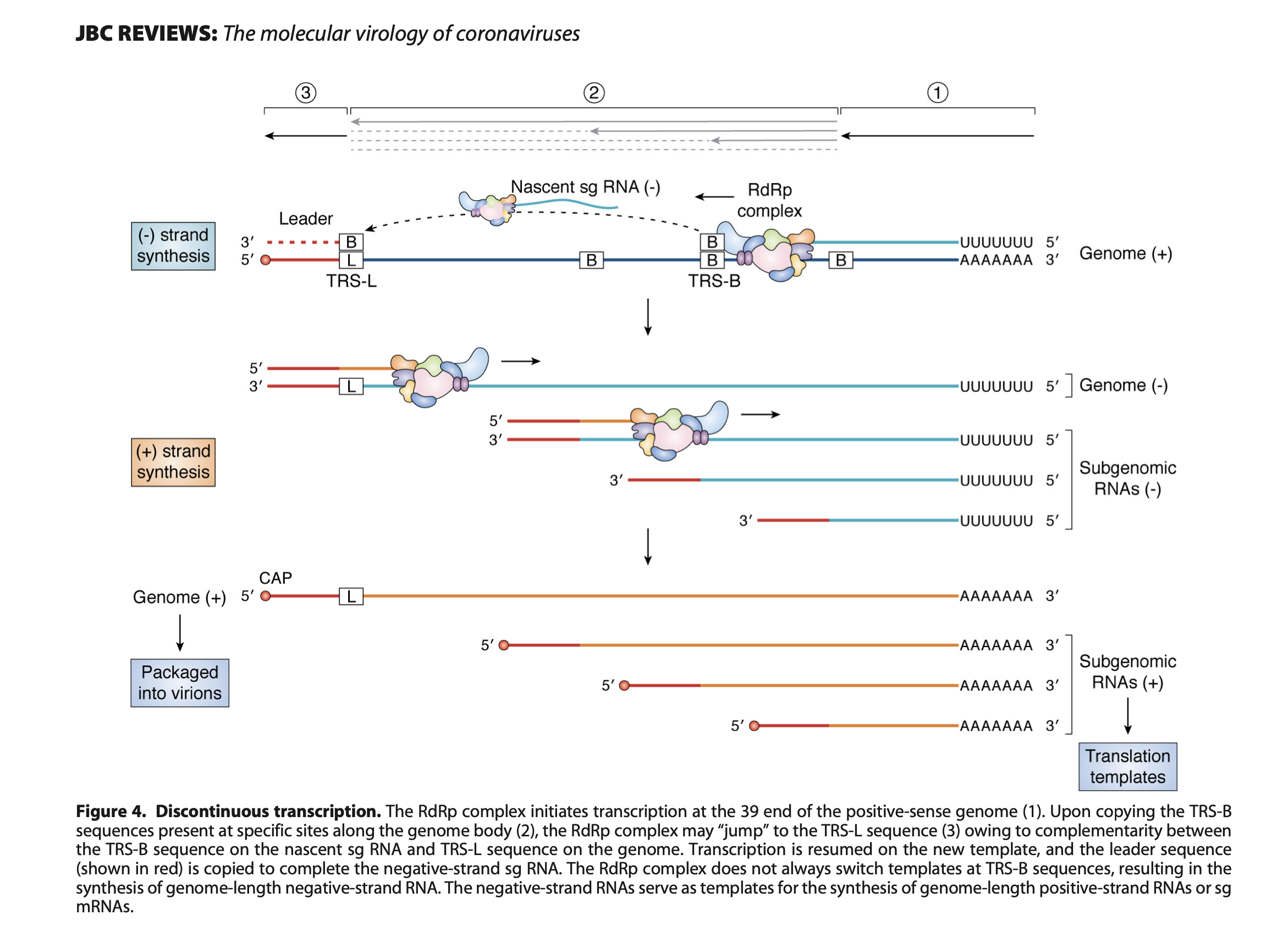
  • sgRNAs are produced through discontinuous transcription during negative-strand synthesis followed by positive-strand synthesis to form mRNA.
  • The resulting sgRNAs contain a leader sequence derived from the 5’ untranslated region of the genome and a transcription regulating sequence (TRS) 5’ of the open reading frame (ORF).
  • The template switch occurs during sgRNA synthesis owing to a conserved core sequence within the TRS 5’ of each ORF (TRS-B, TRS-Body) and the TRS within the leader sequence (TRS-L, TRS-Leader).
  • The conserved core sequence leads to base-pairing between the TRS-L and the nascent RNA molecule transcribed from the TRS-B, resulting in a long-range template switch and incorporation of the 5’ leader sequence.
  • SARS-CoV-2 produces at least nine canonical sgRNAs containing ORFs for four structural proteins (S, spike; E, envelope; M, membrane; N, nucleocapsid) and several accessory proteins (3a, 3b, 6, 7a, 7b, 8, and 10).
• Steps of SARS-CoV-2 Replication:
  1. Attachment: The virion’s spike protein (S) binds to the angiotensin-converting enzyme 2 (ACE2) receptor on the surface of host cells.
  2. Entry: The fusion of viral and host cell membranes leads to the entry of viral RNA genome into the host cell’s cytoplasm.
  3. Translation: The host ribosomes translate the viral RNA into two large polyproteins, pp1a and pp1ab, which are then cleaved by viral proteases into individual nonstructural proteins (nsps). These nsps form the replicase-transcriptase complex (RTC).
  4. Replication: The RTC synthesizes full-length negative-sense RNA molecules using the viral positive-sense RNA as a template.
  5. Transcription: Discontinuous transcription occurs in a nested manner for the synthesis of subgenomic RNAs (sgRNAs). The RTC pauses at the transcription regulatory sequence – body (TRS-B), jumps to the corresponding transcription regulatory sequence – leader (TRS-L), and forms a canonical sgRNA containing both the 5’ leader sequence and the downstream open reading frame (ORF).
     • The RdRp encounters a TRS-B and pauses.
     • The enzyme then switches templates and jumps to the corresponding TRS-L within the leader sequence.
     • Transcription resumes by extending the nascent RNA chain with the leader sequence.
     • The resulting fusion product forms a canonical sgRNA, containing both the 5’ leader sequence and the ORF downstream of TRS-B.
  6. Assembly:
     • Translation of subgenomic mRNAs results in the production of structural and accessory proteins.
     • The nucleocapsid (N) protein binds to the newly synthesized genomic RNA to form a helical ribonucleocapsid.
     • The envelope (E), membrane (M), and spike (S) proteins localize to the endoplasmic reticulum (ER) - Golgi intermediate compartment (ERGIC).
     • Ribonucleocapsid associates with these viral structural proteins, forming a complete virion.
  7. Release: Mature virions are transported via secretory vesicles towards the plasma membrane, where they fuse with the membrane and undergo exocytosis, releasing new virions into the extracellular space.

  In summary, the replication process of SARS-CoV-2 involves multiple stages, including attachment, entry, translation, replication, transcription of subgenomic RNAs, assembly, and release. This process results in the production and release of new viral particles that can infect other cells.

• Beyond the regulation of transcription, sgRNA may also play a role in the evolution of coronaviruses, and the template switching required for sgRNA synthesis may explain the high rate of recombination seen in coronaviruses.

• Previous studies of SARS-CoV-2 sgRNA have used methods that specifically detect expressed RNA, such as direct RNA sequencing of cultured cells infected with SARS-CoV-2 or more traditional total poly(A) RNA-seq. We hypothesized that we could detect and quantify the levels of sgRNA to both identify novel noncanonical sgRNA and provide an estimate of ORF sgRNA expression in SARS-CoV-2 sequence data.

Results

ARTIC network Nanopore sequencing data

To separate gRNA from sgRNA reads, we use the following workflow using Snakemake; raw ARTIC Network Nanopore sequencing reads that pass QC are collected and aligned to the SARS-CoV-2 reference; and reads are filtered out if they are unmapped or supplementary alignments (reads with an alternate mapping location). We do not perform any length filtering. Each read is assigned an amplicon. We search the read for the presence of the leader sequence (5 -AACCAACTTTCGATCTCTTGTAGATCTGTTCT-3) using a local alignment. If we find the leader with a strong match, it is likely that that read is from amplification of sgRNA. We assign reads to an ORF. By using all of this information, we then classify each read into genomic, canonical sgRNA or noncanonical sgRNA and produce summaries for each amplicon and ORF, including normalized pseudoexpression values. sgRNA reads are binned into either high quality (HQ), where the leader alignment score is 50 or more; low quality (LQ), where the leader alignment score is 30 or more; or low, low quality (LLQ), where the read still begins at a known ORF start site.

Illumina sequencing data

Next, we wanted to investigate whether we could use a similar method to Illumina sequencing data. Illumina sequencing data for SARS-CoV-2 has been generated using three main approaches: amplicon based (ARTIC Network), bait capture based, or metagenomics on in vitro samples. Here we describe sgRNA detection in both Illumina bait-based capture and Illumina metagenomic data from in vitro experiments. The reads from these techniques tend to have differing amounts of leader at the 5 end of the reads. This is owing to library preparation methods used in these workflows. We therefore implemented a modified method for detecting sgRNA to ensure that we could capture as many reads originating from sgRNA as possible. In our Illumina implementation , we extract the soft-clipped bases from the 5’ end of reads and use these in a local alignment to the leader sequence. In addition to adjusting the leader detection method, we also process mate pairs, ensuring both reads in the pair are assigned the same status.

Normalization of subgenomic read abundance

In the case of ARTIC Network Nanopore sequencing data. Because we have a median of 258,210 mapped reads for samples from the Sheffield data set, we normalized both gRNA or sgRNA per 100,000 mapped reads (gRNA reads per 100,000 [gRPHT] or sgRNA reads per 100,000 [sgRPHT], respectively).

In our second approach, because of differences in amplicon performance in the ARTIC PCR protocol that lead to coverage differences in the final sequencing data, we determine the amplicon from which the sgRNA has originated, using methods from the ARTIC Network Field Bioinformatics package (2020). We then normalize the sgRNA per 1000 gRNA reads from the same amplicon. If a sgRNA has resulted from more than one amplicon, the resulting normalized counts from each amplicon are summed, giving us sgRNA reads per 1000 gRNA reads (sgRPTg) for every ORF.

For Illumina data, we applied one further normalization technique to allow the normalization of bait-based capture and metagenomic data. (I am curious here why the authors did not report amplicon-based Illumina data) Efficiency of capture varies between probes and designs. For metagenomic data, natural fluctuations in coverage owing to sequence content can exist, therefore, to try and account for this, we took the median coverage for the region around each canonical ORF start site (±20 bp) as the denominator in the nor malization of these data.

Lower limit of detection

In our experience, we generally see much lower total amounts of sgRNA compared with their genomic counterparts; therefore, its detection is likely to suffer when a sample has lower amounts of reads.

The authors downsampled 23 samples that had more than 1 million mapped reads to lower read counts, and found that lower counts of the 5000 and 10,000 reads do not correlate with those generated from 100,000, 200,000, and 500,000 reads (R2<0.7). Samples with 50,000 reads seem to perform well compared with 100,000, 200,000, and 500,000 reads, with an R2 of 0.94, 0.89, and 0.89, respectively.

Methods

Preprocessing

• Nanopore: Pass reads for single isolates are concatenated and aligned to MN908947.3 with minimap2 (v2.17) (-ax map-ont -k 15). It should be noted that adapters or primers are not trimmed. BAM files are sorted and indexed with SAMtools (Li et al. 2009).
• Illumina: Paired-end reads, ideally before trimming, are aligned to MN908974.3 with BWA-MEM (v0.7.17) with the “Y” flag set to use soft clipping for supplementary alignments. BAM files are sorted and indexed with SAMtools.

Periscope: leader identification and read classification

• Nanopore: Reads from the minimap2 aligned BAM file are then processed with pysam (Gilman et al. 2019). If a read is unmapped or represents a supplementary alignment, then it is discarded. Each read is then assigned an amplicon using the “find_primer” method of the ARTIC field bioinformatics package. We search for the leader sequence (5 -AACCAACTTTCGATCTCTTGTAGATCTGTTCT-3 ) with Biopython local pairwise alignment (localms) with the following settings: match +2, mismatch −2, gap -10, and extension -0.1, with score_only set to true to speed up computation. The read is then assigned an ORF using a pybedtools and a BED file consisting of all known ORFs ±10 of the predicted leader/genome transition. We classify reads as a HQ sgRNA if the alignment score is greater than 50 and the read is at a known ORF. If the read starts at a primer site, then it is classified as gRNA; if not, then it is classified as a HQ noncanonical sgRNA supporting read. If the alignment score is greater than 30 but 50 or less and if the read is at a known ORF, then it is classified as a LQ sgRNA. If the read is within a primer site, it is labeled as a gRNA; if not, then it is a LQ sgRNA. Finally, any reads with a score of 30 or less that are at a known ORF are then classified as a LLQ sgRNA; otherwise, they are labeled as gRNA. The following tags are added to the reads for manual review of the periscope calls: XS, alignment score; XA, amplicon; AC, read class; and XO, the read ORF. Reads are binned into qualitative categories (HQ, LQ, LLQ, etc.) because we noticed that some sgRNAs were not classified as such owing to a lower match to the leader. After manual review, they are deemed bona fide sgRNA. This quality rating negates the need to alter alignment score cutoffs continually to find the best balance between sensitivity and specificity. Restricting to HQ data means that sensitivity is reduced but specificity is increased, including LQ calls will decrease specificity but increase sensitivity. Notes: If a read is assigned an ORF but it doesn’t align to the leader sequence it is labelled as gRNA.

• llumina: Reads from the BWA-MEM-aligned BAM file are processed with pysam. If a read is unmapped or represents a supplementary alignment, then it is discarded. The presence of soft clipping at the 5 end of the reads is an indicator that the read could contain the leader sequence so we extract all of the soft clipped bases from the 5 end, additionally including three further bases to account for homology between leader and genome at the N ORF (these bases would therefore not be soft clipped at this ORF). If there are fewer than six extracted bases in total, we do not process that read further as this is not enough to determine a robust match to the leader sequence. With a match score of two and a mismatch score of −2 (gap opening penalty, −20l extension, −0.1), soft clipped bases are aligned to the leader sequence with localms. Soft clipped bases that include the full ≥33 bp of the leader would give an alignment score of 66. Allowing for two mismatches, this gives a “perfect” score of 60. If the number of soft clipped bases is less, then we adjust the “perfect” score in the following way: Perfect Score = (Number of bases soft clipped × 2)−2. This allows for one mismatch. The position of the alignment is then checked; for these bases to be classed as the leader, the alignment of the soft clipped bases must be at the 3′ end. If this is true and (Perfect Score − Alignment Score) ≤ 0, then the read is classified as sgRNA.