Book notes: Coalescent theory: An introduction

The book Coalescent theory: An introduction by John Wakeley stays in my bookshelf for more than 3 years. I have tried started reading it several times, but I always got stuck in the first two chapters. This time I decided to read it for preparing my attendance to the workshop on coalescent theory at the University of Warwick in the next month. Now let us start.

For reference, here is the list of corrections to the book.

1. Gene genealogies

The goal of population genetics is to understand the forces that produce and maintain genetic variation within species. The forces include mutation, recombination, natural selection, population structure, and random transmission of genetic material from parents to offspring. Coalescent theory is a part of theoretical population genetics.

• Nonfunctional parts of the genome are especially informative about ancestry because mutations in these regions accumulate at a more constant rate and are more abundant than those within protein-coding or otherwise functional loci.
• Mutations are rare, so the record of ancestry in DNA is incomplete. Still, when we observe some number of differences between a pair of sequences at the same locus, we know that the time back to their common ancestor must be long enough for the observed number of mutations to have occurred with reasonable probability.
• Coalescent model considers the variation in times to common ancestry, which can be heavily influenced by the population-level process.
• The genetic ancestry of a sample, or the gene genealogy, is the set of ancestral relationships among the members of the sample.
• Gene genealogies are by the nature unobservable, and they are treated as random variables in a statistical setting.
• Thus, while in phylogenetics the tree structure itself is significant, within species it is often the case that particular gene genealogies provide little information about population-level processes and events.

1.1 Genealogies and genealogical thinking

• The shapes of inter-species gene genealogies, often called gene trees, for the most part coincide with the phylogenetic trees of the species from which the samples were taken. In contrast, gene genealogies for samples from a single species are more strongly influenced by the random process of genetic transmission and of birth and death of individuals within populations. The outcome of thess processes is called genetic drift.
• Coalescent genealogies without recombination are rooted bifurcating trees.
• We count a total of $2n-3$ branches in an unrooted tree with $n$ tips. There are $n-1$ coalescent events. The number of internal branches is $n-2$. Internal branches partition the sample into subsets that both contain at least two members (view from the perspective of a unrooted tree).
• Mutations can happen on the branches of the genealogy.
• Because there are $2n-2$ branches in each genealogy, a single mutation placed on a genealogy will produce one of $2n-2$ possible patterns. Or $2n-3$ in a unrooted tree.
• We can access compatibility between two polymorphic sites directly, by comparing the subsets each makes of the sample. If both subsets at one site overlap with both subsets at the other site, then they are incompatible.

1.2 Mutation and mutation models

Mutation is the bridge from genealogies to genetic data because the structure of the genealogy, in which each branch divides the sample into two groups, is revealed only if polymorphisms exist among the sampled sequences.

• Mutation models can be divided roughly into two groups: allele-based models and nucleotide-sequence models. Allele-based models typically do not encode any information about the historical relationships among alleles in a sample, whereas models for nucleotide sequences naturally generate such information in the patterns of polymorphism they among sites in the sample.
• An important simplifying assumption in modelling mutations within the coalescent is that all variation is selectively neutral, meaning that mutation does not affect the reproductive success of organism and has no influence on the genealogy structure. Thus, the genealogical process and mutation process can be separated, and any mutation model can in principle be applied by considering changes along the branches of each genealogy. In practice, analytical results can be easily found under the infinite-alleles and infinite-sites models, while other models are generally implemented using computer simulations.
• The infinite-sites assumption may be acceptable for nuclear DNA sequences as a first approximation, when the mutation rate is low. However, if a great deal of time has passed between the ancestor and its descendant, it will be likely that multiple mutations will have occurred. In this case, we must use detailed models of DNA sequence change and take the possibility of homoplasy, or convergence in state, into account.

1.3 Measures of DNA sequence polymorphism

There are some summary statistics that can be used to quantify levels of genetic variation in DNA sequences.

Three historical important summary statistics are: the number of segregating sites, the average number of pairwise differences, and the site frequencies or site-frequency spectrum.

• The number of segregating sites ($S$, Watterson, 1975) is the number of sites in the sample that are polymorphic. It can be affected by the length of the sequence, the mutation rate, and the sample size.
• The average number of pairwise differences ($\pi$, Tajima, 1983) is the average number of differences between pairs of sequences in the sample. It is should be less affected by sample size.
• Site frequencies ($\eta_i$) provide an intermediate measure, one between the total data and the extreme summaries $S$ and $\pi$.
• $S$ and $\eta_i$ count each mutation exactly once, whereas $\pi$ weights sites depending on how the branch where the mutation occurred, or the site itself, divides the sample. $\pi$ is largest when the mutation frequency is in the middle ($i=n/2$), and smallest when it is at the ends ($i=1$), so the middle-frequency sites contribute disproportionately to $\pi$.
• The distribution of the polymorphism among chromosomes, or haplotypes, is sacrificed in the summary statistics.

2. Probability theory

2.1 Fundamentals

We skipped some basic concepts, and only recorded some important concepts.

• $Var[X] = E[X^2] - E[X]^2$
• $Cov[X,Y] = E[XY] - E[X]E[Y]$
• $Var[X+Y] = Var[X] + Var[Y] + 2Cov[X,Y]$

Considering sums of two random variables $Y=X_1+X_2$, in the case where the $X_i$ are independent, the distribution of the sum is the convolution of the distributions of the $X_i$. In the discrete case, we have $P(Y=y) = \sum_i P(X=x)P(Y=y-i)$.

If we have $Y=X_1 + X_2 + \cdots + X_K$ where $K$ is a random variable. If $X_1, X_2, \cdots, X_K$ are independent and identically distributed, then $E[Y] = E[X]E[K]$ and $Var[Y] = E[X^2]Var[K] + Var[X]E[K]^2$.

• The binomial distribution: How many successes in $n$ trials. (number of successes)
• The geometric distribution: How many trials until the first success. (waiting time)
• The Poisson distribution: How many events in a fixed interval of time. (number of events)
• The exponential distribution: How long until the next event. (waiting time)
• The gamma distribution: How long until the $k$-th event. (waiting time)

2.2 Poisson processes

• The sum of independent Poisson random variables is another Poisson process whose rate is equal to the sum of the individual rates.
• The probability that the first event in a Poisson process is of a particular type is the relative rate of that event.
• The time to first event in a Poisson process is exponentially distributed with rate equal to the sum of the rates of the individual events.
• The number of events required to see a particular event type is geometrically distributed with success probability equal to the relative rate of that event.
• Convolutions of exponential distributions are gamma distributions. If $\lambda_i \neq \lambda_j$, then it is necessary to take a series of convolutions. $f_{T_1+T_2}$ will be a weighted sum of the distributions $f_{T_1}$ and $f_{T_2}$.

3. The coalescent

3.1 Population genetic models

3.1.1 The Wright-Fisher model

The Wright-Fisher model is a discrete-time model of genetic drift. It is a model of a single, isolated, randomly mating population of constant size. The population is diploid (no males and females), and the number of offspring produced in each generation is fixed. The model is a Markov chain, and the state space is the set of all possible allele frequencies. $K_t$ is the number of copies of allele $A_1$ in the population at time $t$.

• The probability that a gene with $i$ copies in the current generation being found in $j$ copies in the next generation is given by the binomial distribution.
• The heterozygosity of the population $H$ is the probability that two randomly chosen genes are different. $H_0 = 2p_0(1-P_0)$ is the heterozygosity at generation 0. The expected heterozygosity is $E[H_t] = H_0(1-\frac{1}{N})^t\approx H_0e^{-t/N}$. We see that the heterozygosity decays exponentially with time. The decrease of heterozygosity is a common measure of genetic drift, and we say that the drift occurs at a rate of $1/N$ per generation.

3.1.2 The Moran model

The Moran model is important for two reasons: 1. it applies to organisms in which generations are overlapping, and 2. mathematically, many results can be derived exactly under the Moran model that are available only approximately under the Wright-Fisher model.

In the Moran model, one of just three things must happen in one time unit: allele $A_1$ increases by one, allele $A_2$ increases by one, or the counts stay the same.

As in the Wright-Fisher model, random genetic drift leads to variation in the number of copies of an allele in the population.

The expected heterozygosity is $E[H_t] = H_0(1-\frac{2}{N^2})^t\approx H_0e^{-2t/N^2}$. The rate of genetic drift per time is $2/N^2$ per generation. If we assume the life span of an individual has mean $N$ generation, the rate for per generation is $2/N$, which is twice as fast as the Wright-Fisher model. This is interesting from a biological perspective, because it means that differences in breeding structure (overlapping generations or not) can have effects on the rate of genetic drift.

3.2 The standard coalescent model

This whole section is way too technical for me and I should probably read it again some time later.

Basically it first introduce Kingman’s coalescent, which is a model of the genealogy of a sample of genes from a population of constant size. In the model, as $N$ goes to infinity, the coalescence times $T_i$ are independent and exponentially distributed with rate $\binom{i}{2}$ (a Poisson process in which each of the $\binom{i}{2}$ pairs of lineages has the same rate $\lambda = 1$ of coalescence). The probability that $k$ lineages coalesce in a time interval of length $t$ is given by the Poisson distribution with mean $\binom{k}{2}t$.

In Sections 3.2.1 and 3.2.2, the author showed the Wright-Fisher model and the Moran model can be approximated by the Kingman’s coalescent model. The Wright-Fisher model is approximated by the Kingman’s coalescent model when $N$ is large and the Moran model is approximated by the Kingman’s coalescent model when $N$ is large and the number of generations is large.

In Section 3.2.3, the author discussed breeding structure and exchangeability. Exchangeability means identically distributed but not independent. Here in a exchangeable-type population model, the number of offspring of individuals in the population is exchangeable, but not independent, as they must sum to $N$. From a biological standpoint, exchangeability means that there can be no transmission of reproductive potential from parents to offspring, nor can there be any correlations in reproductive potential due to other factors, such as geographic location or social status.

3.3 Some properties of the coalescent genealogies

3.3.1 Two measures of the size of a genealogy

The coalescence times $T_i$ are (1) independent of one another and (2) independent of the branching structure of the genealogy.

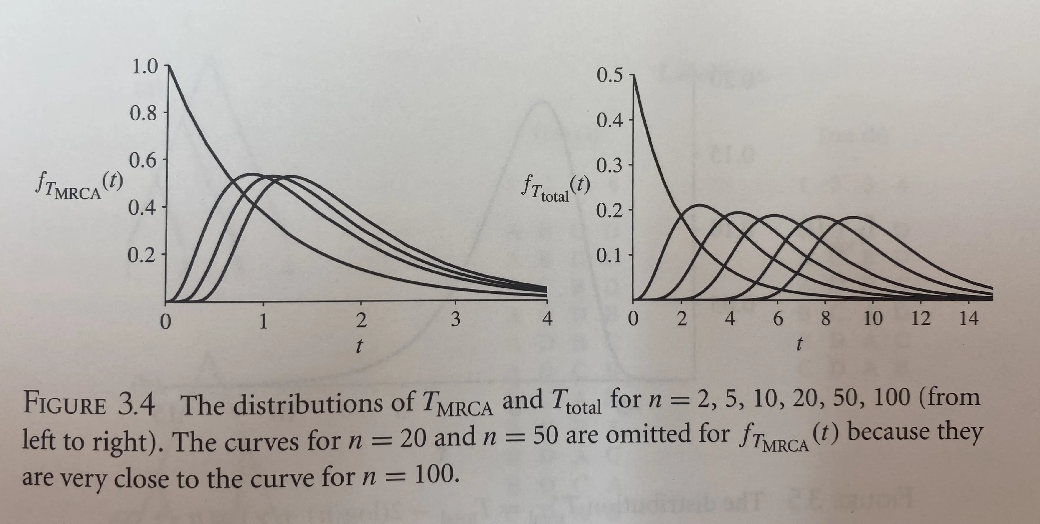
$E[T_{MRCA}]$ is close to its asymptotic value of 2 even for moderate $n$. The mean of 2 corresponds to a period of $2N$ generations under the haploid Wright-Fisher model. $E[T_{total}]$ increase without bound as $n$ increases, but it dose so more slowly for larger $n$.

As shown in the below figure, the asymmetry of $f_{T_{MRCA}}(t)$ (e.g., that the mode is less than the mean) reflects the strong influence of the most ancient coalescence time, $T_2$, which makes up a significant fraction of $T_{MRCA}$ even when $n$ is large.

3.3.2 The branching structure of genealogies

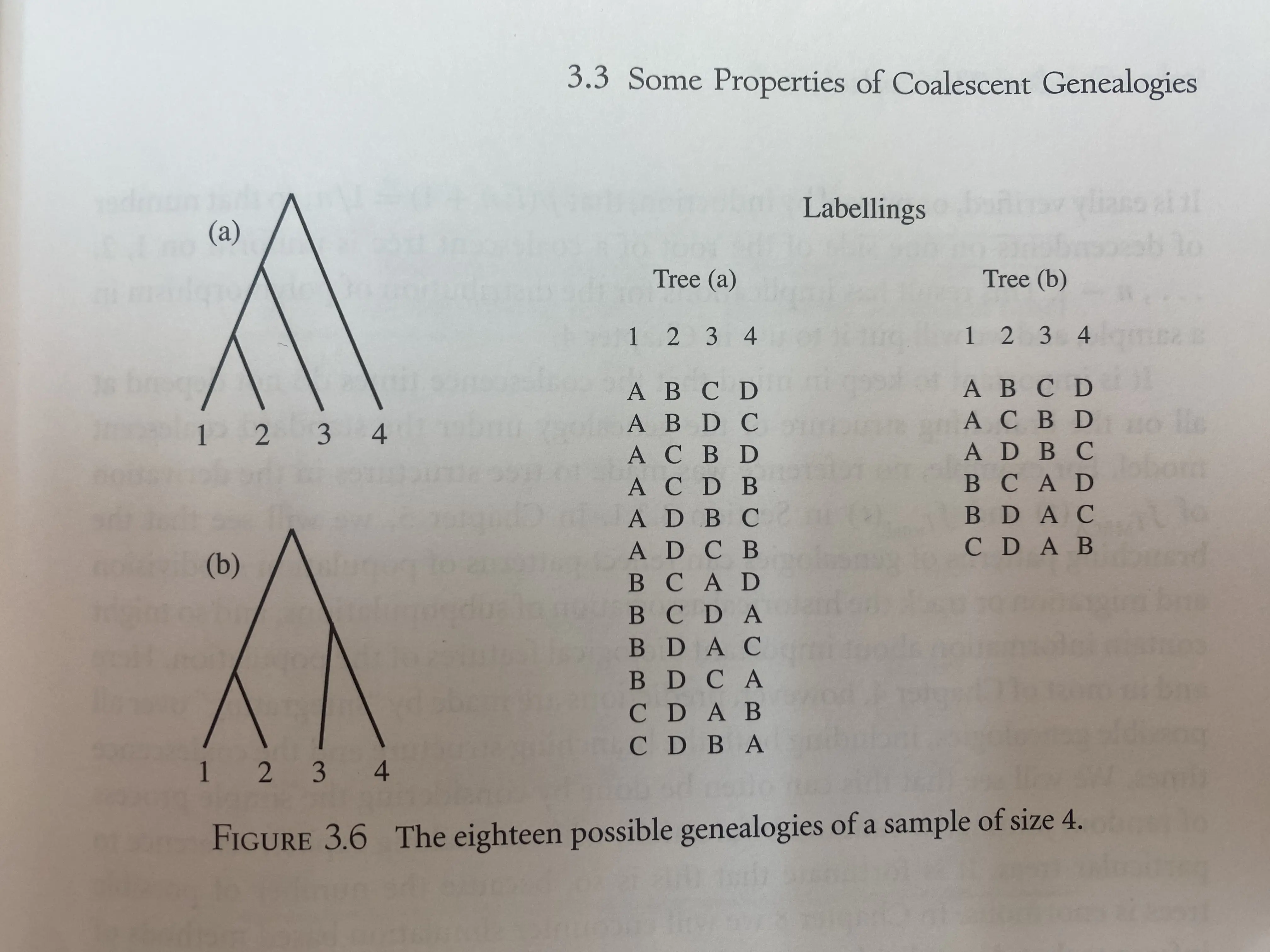
The number of possible tree structures (genealogies) can be obtained by considering the number of possible coalescent events at each step toward the MRCA. Beginning with the present-day sample of $n$ items, whenever there are $i$ lineages present there are $\binom{i}{2}$ possible pairs of lineages to coalesce. The total number of these random-joining trees is given by \(\prod_{i=2}^{n}\binom{i}{2} = \frac{n!(n-1)!}{2^{n-1}}.\)

For a unrooted tree, the number of possible tree topologies is $(2n-5)!!$, or the product of all odd numbers from $2n-5$ down to 1.

3.4 Human-neanderthal couples?

This example and its probability inference is super interesting. It is also very hard to follow. I should read it again later.

4. Neutral genetic variation

Time for coalescent process is measured in $N_e = N/\sigma^2$ generations, and mutation rates are measured on a timescale proportional to this. For historical reasons, population geneticists introduce an extra factor of 2, and use the mutation parameter $\theta = 2N_e\mu$, in which $\mu$ is the mutation rate per site per generation. In the Writh-Fisher model, where $N_e = N$, mutations occur with rate $\theta/2$ per generation. Given that the length of a genealogy is equal to $t$, the number $K$ of mutations, is itself Poisson distributed with mean $\theta t/2$: \(P(K=k|t) = \frac{(\theta t/2)^k}{k!}e^{-\theta t/2}.\) and the expected number of mutations is $E[K] = \theta t/2$.

Neutral mutations, which do not affect fitness, do not affect the shape of the genealogy.

4.1 The infinite-sites model and measures of DNA sequence polymorphism

4.1.1 The number of segregating sites