This is the BEAST2 book by Alexei J. Drummond and Remco R. Bouckaert. I will focus on the Part I of this book, which is the theory part. Part III also seems to be interesting, it is on programming.

Below are some notes.

Introduction

Molecular phylogenetics

• The statistical treatment of phylogenetics was made feasible by Felsenstein (1981), who described a computationally tractable approach to computing the probability of the sequence alignment given a phylogenetic tree and a model of molecular evolution, $Pr{D\vert T,\Omega}$. This quantity is known as the phylogenetic likelihood of the tree and can be efficiently computed by the peeling algorithm.
• A continuous-time Markov process (CTMP) can be used to describe the evolution of a single nucleotide, assuming iid of the sites, this can be extended to multiple sequence alignment.
• Bayesian inference have great flexibility in describing prior knowledge, and it can apply to complex highly parametric models via MCMC.

Coalescent theory

• A gene tree is estimated from individuals sampled from a population, the size of the population can be estimated using Kingman’s coalescent model.
• Genealogy-based population genetics methods can infer many parameters governing molecular evolution and population dynamics, including effective population size, rate of population growth/decline, migration rates, population structure, recombination rates and reticulate ancestry.
• Kingman’s coalescent.
• Incomplete lineage sorting (ILS) is commonly modeled using the multispecies coalescent framework, which integrates a population-level coalescent process (gene tree) into a phylogenetic (species) tree.

Virus evolution and pholodynamics

• Because RNA viruses evolve so quickly, the “evolutionary clock” (the genetic changes in virus populations) runs at a similar pace to the “ecological clock” (the spread and decline of infections, changes in host populations, and alterations in transmission routes).
• Neutral genetic variation—mutations not heavily influenced by natural selection—provides a molecular record of the virus’s past.

Before and beyond tress

• Sequence alignment:
  • ClustalW and ClustalX uses a guide tree constructed by a distance-based method to progressively construct MSA via pairwise alignment. This guide tree may be a bias if you aim to reconstruct the phylogeny using the MSA.
  • T-coffee builds a library of pairwise alignments to construct a MSA.
  • MUSCLE and MAFFT are suitable for high-throughput MSA.
  • Statistical alignment reconstructs the MSA and the phylogeny simultaneously, using a probabilistic model of sequence evolution.
• Ancestral recombination graph (ARG) is a generalization of a genealogy that includes recombination events.

Probability and Bayesian inference

• Bayes’ formula: $P(\theta\vert D) = \frac{P(D\vert \theta)P(\theta)}{P(D)}$.
• In a phylogenetic context, $f(\theta\vert D) = \frac{Pr(D\vert\theta)f(\theta)}{Pr(D)}$, where D is the sequence data, $\theta$ is the set of parameters, including the tree, substitution model parameters, clock rates, etc. $f(\theta\vert D)$ is the posterior distribution, $Pr(D\vert \theta)$ is the likelihood, $f(\theta)$ is the prior distribution, and $Pr(D)$ is the marginal likelihood.
• The marginal likelihood is the probability of the data averaged over all possible values of the parameters, $Pr(D) = \int Pr(D\vert \theta)f(\theta)d\theta$. It is almost always intractable to compute, but it can be estimated using MCMC.
• Non-informative priors hold a natural appeal, but they can be improper in a formal sense if they do not integrate to 1 over the parameter space. Such improper priors are extremely dangerous in a Bayesian analysis, as they can lead to improper posteriors.
• In MCMC, the new state is accepted with probability $\alpha = min{1, \frac{f(\theta’\vert D)}{f(\theta\vert D)}}$, where $\theta’$ is the proposed new state. This algorithm assumes that the proposal distribution is symmetric, where $q(\theta’\vert \theta) = q(\theta\vert \theta’)$.
• Effective sample size (ESS) is a measure of the number of independent samples in a chain, accounting for autocorrelation.
• The Metropolis-Hastings algorithm is a generalization of the Metropolis algorithm that allows for asymmetric proposal distributions. MCMC maintains reversibility by factoring in a Hastings ratio, $\alpha = min{1, \frac{f(\theta’\vert D)q(\theta\vert \theta’)}{f(\theta\vert D)q(\theta’\vert \theta)}}$.
• Gibbs sampler is a special case of the Metropolis-Hastings algorithm, where the proposal distribution is the conditional distribution of each parameter given the others.
• When the parameter space is not of a fixed dimension, reversible-jump MCMC or Bayesian variable selection (BSVS) can be used to explore the space of models with different numbers of parameters.
• Bayes factors are used to compare the fit of different models to the data, $BF = \frac{Pr(D\vert M_1)}{Pr(D\vert M_2)}$, which rely on the marginal likelihoods of the models.
• Path sampling is a computational technique used in Bayesian phylogenetic inference to estimate the marginal likelihood by slowly “turning on” the likelihood function. By evaluating how the expected log-likelihood changes as you go from the prior distribution ($β=0$) to the posterior distribution ($β=1$), you obtain a numerical approximation of the marginal likelihood—an essential quantity for rigorous Bayesian model comparison.
• Maximum likelihood methods find the $max_\theta Pr(D\vert \theta)$. Bayesian inference finds the posterior distribution $f(\theta\vert D)$.
• The posterior distribution lets you reason about how plausible different parameters are, not just the single best estimate.

Evolutionary trees

Types of trees

• A rooted binary tree of $n$ leaves has $2n-1$ nodes (both internal nodes and tips) and $2n-2$ branches.
• Multifurcating trees (as opposed to bifurcating/binary trees) are those that have one or more polytomies.
• In time trees, the times of the internal nodes are called divergence times, ages or coalescent times, while the times of the leaves are known as tip times or sampling times.
• When inferring rooted tress, we link the amount and duration of evolution. If amount and duration is the same, we assume a strict clock model. If there is large variance between the two, we assume a relaxed clock model.
• Since in a time-tree node heights correspond to the ages of the nodes, such rooted tree models have fewer parameters than unrooted tree models, approaching roughly half for large number of taxa (for $n$ taxa, there are $n-1$ node heights for internal nodes and a few parameters for the clock model, but $2n-3$ internal nodes in an unrooted tree).

Counting trees

• The number of tip-labelled rooted binary trees for $n$ taxa is: \(T_n = \prod_{k=2}^n {(2k-3)} = (2k-3)(2k-5)...(7)(5)(3)(1).\)

• The number of unlabelled rooted tree shapes, the number of labelled rooted trees, the number of labelled ranked trees (on contemporaneous tips) and the number of fully ranked trees (on distinctly timed tips) as a function of the number of taxa, $n$

  n	#shapes	#trees ($T_n$)	#ranked trees ($R_n$)	#fully ranked trees ($F_n$)
  2	1	1	1	1
  3	1	3	3	4
  4	2	15	18	34
  5	3	105	180	496
  6	6	945	2,700	11,056
  7	11	10,395	56,700	349,504
  8	23	135,135	1,587,600	14,873,104
  9	46	2,027,025	57,153,600	819,786,496
  10	98	34,459,425	2,571,912,000	56,814,228,736

• The number of tree shapes (or unlabelled rooted tree topologies) of $ n $ taxa, $ a_n $, is given by (Cavalli-Sforza and Edwards 1967):

  \[a_n = \begin{cases} \sum_{i=1}^{(n-1)/2} a_i a_{n-i}, & \text{if } n \text{ is odd} \\ a_1 a_{n-1} + a_2 a_{n-2} + \dots + \frac{1}{2}a_{n/2}(a_{n/2} + 1), & \text{if } n \text{ is even}. \end{cases}\]

• Ranked tree differ from unranked trees in that the internal nodes are ordered, and fully ranked trees are those where the tips are ordered by time of sampling.

• There are more ranked trees than rooted tree topologies, and they are important because many natural tree priors are uniform on ranked trees rather than tree shapes. The number of ranked trees of $ n $ contemporaneous taxa, $F(n) = \vert R_n\vert $, is:

  \[F(n) = |R_n| = \prod_{k=2}^n \binom{k}{2} = \frac{n!(n-1)!}{2^{n-1}}.\]

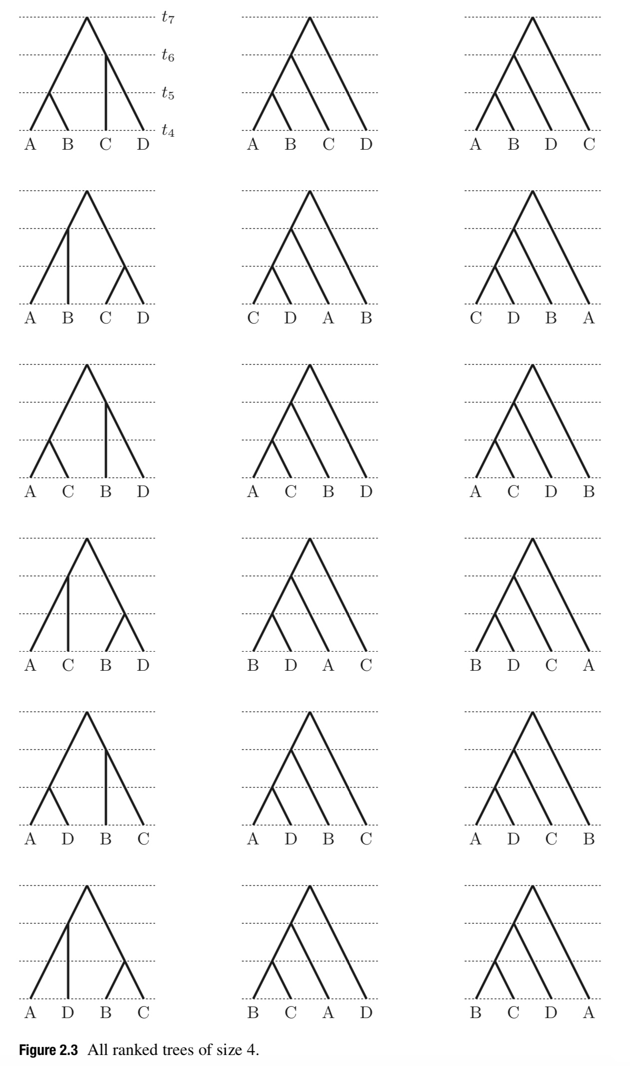
• All ranked trees with four tips are shown in Figure 2.3. When a tree has non-contemporaneous times for the sampled taxa, we term the tree fully ranked (Gavryushkina et al. 2013), and the number of fully ranked trees of $ n $ tips can be computed by recursion:

  \[F(n_1, \dots, n_m) = \sum_{i=1}^{n_m} \frac{|R_{n_m}|}{|R_i|} F(n_1, n_2, \dots, n_{m-2}, n_{m-1} + i),\]

  where $ n_i $ is the number of tips in the $ i $-th set of tips, grouped by sample time (see Gavryushkina et al. 2013 for details).

  

The Coalescent

• The Wright-Fisher model in its simplest form assumes (1) constant population size $N$, (2) discrete generations, (3) complete mixing.

• The below example shows when two individuals sampled from the current generation traced back in time. The probability of coalescence at $t$ generations is $Pr(t)=\frac{1}{N}(1-\frac{1}{N})^{t-1}$. The expected waiting time for coalescence is $E(\tau_k)=\frac{N}{K\choose2}$, where $k$ is the number of lineages. { width=500pt }
• Kingman shows that as $N$ grows the coalescent process converges to a CTMC, where the waiting time for coalescence is exponentially distributed with rate $\frac{K\choose2}{N}$.
• Effective population size may be useful for comparing different populations, however see Gillespie (2001) for an argument that these neutral evolution models are irrelevant to much real data because neutral loci will frequently be sufficiently close to loci under selection, that genetic draft and genetic hitchhiking will destroy the relationship between population size and genetic diversity that coalescent theory relies on for its inferential power.

Coalescent with changing population size in a well-mixed population

• Parametric models with a pre-defined population function, such as exponential growth, expansion model and logistic growth models can easily be used in a coalescent framework.
• Non-parametric models, such as skyline plot models treat the coalescent intervals as separate segments. The generalized skyline plot can group the intervals according to the small-sample Akaike information criterion (AICc). Generalized skyline plots can be implemented in a Bayesian framework, which simultaneously infers the sample genealogy, the substitution parameters and the population size history.
• The Bayesian skyline plot analysis of a data set collected from a pair of HIV-1 donor and recipient was used to reveal a substantial loss of genetic diversity following virus transmission (Edwards et al. 2006). A further parametric analysis assuming constant population size in the donor and logistic growth model in the recipient estimated that more than 99% of the genetic diversity of HIV-1 present in the donor is lost during horizontal transmission.
• Serially sampled coalescent: The tree shape probability is conditioned on sampled $\tau$ time:
• 

Modelling epidemic dynamics using coalescent theory

• SIR type models can be combined with coalescent theory to model the spread of infectious diseases. Currently, the probabilities of phylogenetic trees can only be solved analytically for small host population sizes in the simplest endemic setting (SI and SIS) (Leventhal et al. 2014).
• Recall that the coalescent calculates the probability density of a tree given the coalescent rate. The coalescent rate for $k$ lineages is $k\choose2$ times the inverse of the product of effective population size $N_e$ and generation time $g_c$. Volz (2012) proposed a coalescent approximation to epidemiological models such as the SIR, where the effective population size $N_e$ is the expected number of infected individuals through time, and the generation time $g_c$.

Birth-death models

• In coalescent models, coalescent times only depend on deterministic population size, meaning population size is the only parameter in the coalescent. If the population size is stochastic and small, the coalescent model may not be appropriate. Birth-death models can be used to model the population size as a stochastic process.

Constant-rate birth-death models

• The continuous-time constant-rate birth–death process is a birth–death process which starts with one lineage at time $z_0$ in the past and continues forward in time with a stochastic rate of birth ($λ$) and a stochastic rate of death ($μ$) until the present (time $0$). At present, each extant lineage is sampled with probability $ρ$.
• The constant-rate birth–death model with $μ = 0$ and $ρ = 1$, i.e. no extinction and complete sampling, corresponds to the well-known Yule model (Edwards 1970; Yule 1924).
• The three parameters $λ, μ, ρ$ are non-identifiable, meaning that the probability density of a time-tree is determined by the two parameters $λ− μ$ and $λρ$ (the probability density only depends on these two parameters if the probability density is conditioned on survival or on $n$ samples (Stadler 2009)). Thus, if the priors for all three parameters are non-informative, we obtain large credible intervals when estimating these parameters
• One difference between the constant-rate birth–death process limit and the coalescent is that the birth–death process induces a stochastically varying population size while classic coalescent theory relies on a deterministic population size.

Time-dependent birth-death models

• The piecewise constant birth–death process is analogue to the coalescent skyline plot where the population size is piecewise constant, thus we call this model the birth–death skyline plot (Stadler et al. 2013). The birth–death skyline plot has been used, for example, to reject the hypothesis of increased mammalian diversification following the K/T boundary (Meredith et al. 2011; Stadler 2011).

Serially sampled birth-death models

• Since in the previous section we only defined a sampling probability $ρ$ at present, the birth–death model only gives rise to time-trees with contemporaneous tips. Stadler (2010) extended the constant rate birth–death model to account for serial sampling by assuming a sampling rate $ψ$. This means that each lineage is sampled with a rate $ψ$ and it is assumed that the lineage goes extinct after being sampled.

Trees within trees

The multispecies coalescent

• So far we assumed that the genealogy equals the species or transmission tree. However, this is an approximation. The genealogy is actually embedded within the species/transmission tree.
• The multispecies coalescent model can be used to estimate the species time-tree $g_S$, together with ancestral population sizes $N$, given the sequence data from multiple genes, whose gene trees may differ due to incomplete lineage sorting (Pamilo and Nei 1988).

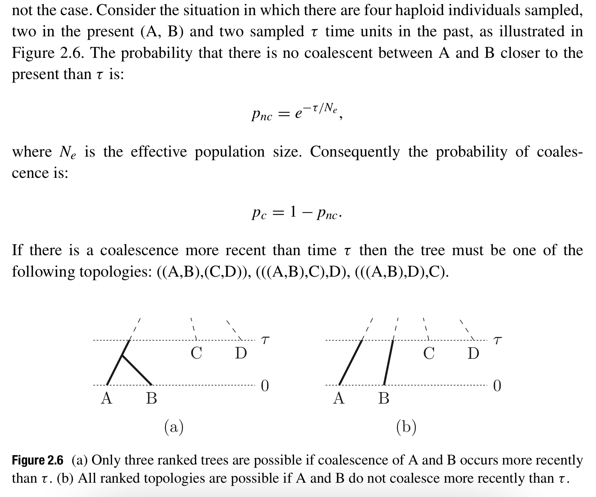
Viral transmission histories

• Nested time-trees can be estimated from a single data set is in the case of estimating transmission histories from viral sequence data, where the nested time-tree is the viral gene tree, and the encompassing tree is the tree describing transmissions between hosts (Leitner and Fitch 1999).
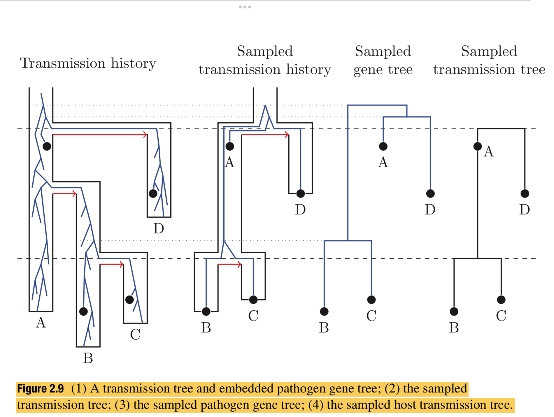
• The natural generative model at the level of the host population is a branching process of infections, where each branching event represents a transmission of the disease from one infected individual to the next, and the terminal branches of this transmission tree represent the transition from infectious to recovery or death of the infected host organism. For multicellular host species there is an additional process of proliferation of infected cells within the host’s body (often restricted to certain susceptible tissues) that also has a within-host branching process of cell-to-cell infections. This two-level hierarchical process can be extended to consider different infectious compartments at the host level, representing different stages in disease progression, and/or different classes of dynamic behaviour among hosts.
• Accepting the above as the basic schema for the generative process, one needs to also consider a typical observation process of an epidemic or endemic disease. It is often the case that data are obtained through time from some fraction, but not all, of the infected individuals. Figure 2.9 illustrates the relationship between the full transmission history and the various sampled histories.
• 
• MASTER/REMASTER can model this schema (combining both the generative and observational processes).

Substitution and site models

• Hamming distance tend to underestimate the number of substitutions, because it does not account for multiple substitutions at the same site.
• Distance correction requires an explicit model of substitution, such as the Jukes-Cantor model. Under JC69, an estimate for the evolutionary distance between two sequences is $d = -\frac{3}{4}ln(1-\frac{4}{3}p)$, where $p$ is the proportion of sites that differ between the two sequences. For $p=0.4$, $\hat{d} \approx 0.571605$. This is an estimate of the expected number of substitutions per site.

Continuous-time Markov process

• Assuming that the Markov process is in state $i \in {A, C, G, T}$ at time $t$, then in the next small moment, the probability that the process transitions to state $j \in {A, C, G, T}$ is governed by the instantaneous transition rate matrix $Q$: \(Q = \begin{bmatrix} \cdot & q_{AC} & q_{AG} & q_{AT} \\ q_{CA} & \cdot & q_{CG} & q_{CT} \\ q_{GA} & q_{GC} & \cdot & q_{GT} \\ q_{TA} & q_{TC} & q_{TG} & \cdot \end{bmatrix}\)

• The total flow out of nucleotide state $i$ and are thus negative. At equilibrium, the total rate of change per site per unit time is thus: \(\mu = -\sum_i \pi_i q_{ii},\) where $π_i$ is the probability of being in state i at equilibrium, so that $μ$ is just the weighted average outflow rate at equilibrium.

• The transition probability matrix, $P(t)$, provides the probability for being in state $j$ after time $t$, assuming the process began in state $i$: \(P(t) = \exp(Qt).\)

DNA models

• All transition probabilities will asymptote equilibrium base frequency (e.g., $\frac{1}{4}$ if base frequencies are equal) for very large $d$.
• Jukes-Cantor: only one parameter, the rate of substitution, $\mu$, which is the same for all transitions. The JC69 model is a special case of the general time-reversible model, where the rate matrix is symmetric, $Q_{ij} = Q_{ji}$.

• K80 (Kimura): The model assumes base frequencies are equal for all characters, only one free parameter, the transition/transversion ratio, $\kappa$. \(Q = \beta \begin{bmatrix} -2 - \kappa & 1 & \kappa & 1 \\ 1 & -2 - \kappa & 1 & \kappa \\ \kappa & 1 & -2 - \kappa & 1 \\ 1 & \kappa & 1 & -2 - \kappa \end{bmatrix}.\)

• F81 (Felsenstein 1981): Allows for unequal base frequencies ($\pi_A \neq \pi_C \neq \pi_G \neq \pi_T$), three free parameters, since the constraint that the four equilibrium frequencies must sum to 1 ($\pi_A + \pi_C + \pi_G + \pi_T = 1$). \(Q = \beta \begin{bmatrix} \pi_A - 1 & \pi_C & \pi_G & \pi_T \\ \pi_A & \pi_C - 1 & \pi_G & \pi_T \\ \pi_A & \pi_C & \pi_G - 1 & \pi_T \\ \pi_A & \pi_C & \pi_G & \pi_T - 1 \end{bmatrix}.\)

• HKY (Hasegawa, Kishino, and Yano 1985): combines the K80 and F81 models, allowing both unequal base frequencies and a transition/transversion ratio. The transition probabilities for the HKY model can be computed and have a closed-form solution, but it is rather long-winded. \(Q = \beta \begin{bmatrix} \cdot & \pi_C & \kappa \pi_G & \pi_T \\ \pi_A & \cdot & \pi_G & \kappa \pi_T \\ \kappa \pi_A & \pi_C & \cdot & \pi_T \\ \pi_A & \kappa \pi_C & \pi_G & \cdot \end{bmatrix}.\)

• GTR (General Time Reversible): the most general time-reversible stationary CTMP for describing the substitution process. The Q matrix is: \(Q = \beta \begin{bmatrix} \cdot & a\pi_C & b\pi_G & c\pi_T \\ a\pi_A & \cdot & d\pi_G & e\pi_T \\ b\pi_A & d\pi_C & \cdot & \pi_T \\ c\pi_A & e\pi_C & \pi_G & \cdot \end{bmatrix}.\)

Codon models

• Codon models (Goldman and Yang 1994; Muse and Gaut 1994) have some key features:
  • a 61-codon state space (excluding the three stop codons);
  • a zero rate for substitutions that changed more than one nucleotide in a codon at any given instant (so each codon has nine immediate neighbors, minus any stop codons);
  • a synonymous/nonsynonymous bias parameter making synonymous mutations, that is mutations that do not change the protein that the codon codes for, more likely than nonsynonymous mutations.

• Given two codons $i = (i_1, i_2, i_3)$ and $j = (j_1, j_2, j_3)$, the Muse–Gaut-94 codon model has the following entries in the $Q$ matrix:

  \[q_{ij} = \begin{cases} \beta \omega \pi_{jk} & \text{if nonsynonymous change at codon position } k \\ \beta \pi_{jk} & \text{if synonymous change at codon position } k \\ 0 & \text{if codons } i \text{ and } j \text{ differ at more than one position} \end{cases}\]

  In addition, the Goldman–Yang-94 model includes a transition/transversion bias giving rise to entries in $Q$ as follows:

  \[q_{ij} = \begin{cases} \beta \kappa \omega \pi_j & \text{if nonsynonymous transition} \\ \beta \omega \pi_j & \text{if nonsynonymous transversion} \\ \beta \kappa \pi_j & \text{if synonymous transition} \\ \beta \pi_j & \text{if synonymous transversion} \\ 0 & \text{if codons differ at more than one position} \end{cases}\]

Felsenstein’s likelihood

• How the likelihood of a phylogenetic tree is computed given sequence data, a tree topology, and a substitution model.

  Key Points: Felsenstein’s Likelihood

1. Definition of the Problem
   • The likelihood $L(g)$ of a phylogenetic tree $g$ is the probability of the observed sequence data $D$, given the tree $g$ and the substitution model parameters $\Omega$: \(L(g) = \Pr(D|g, \Omega).\)
   • Parameters $\Omega$ include:
     • $Q$: Substitution model parameters (rate matrix).
     • $\mu$: Overall substitution rate.
2. Unknown Ancestral Sequences
   • $D_Y$ represents an $(n-1) \times L$ matrix of unknown ancestral sequences at the internal nodes of the tree.
   • The likelihood is computed by summing over all possible ancestral sequences $D_Y$, a process denoted as $\mathcal{C}^{(n-1)L}$.
3. Substitution Probabilities
   • Substitution probabilities along a branch $(i, j)$ are computed using a Continuous-Time Markov Process (CTMP).
   • For a substitution from state $c$ to $c’$ over time $t_i - t_j$, the probability is: \(\Pr(s_{j,k} = c' | s_{i,k} = c) = [e^{Q\mu(t_i - t_j)}]_{c,c'}.\)
4. Likelihood Formula
   • The likelihood of the data is expressed as: \(\Pr(D|g, \Omega) = \sum_{D_Y \in \mathcal{C}} \prod_{(i,j) \in R} \prod_{k=1}^L \left[ e^{Q\mu(t_i - t_j)} \right]_{s_{i,k}, s_{j,k}}.\)
     • $R$: Set of all branches in the tree.
     • The sum is over all possible ancestral sequences $D_Y$.
5. Practical Computation
   • Summing over all ancestral sequences $D_Y$ is computationally intensive.
   • Felsenstein’s pruning algorithm enables efficient computation by recursively marginalizing over ancestral states, reducing complexity.

Rate variation across sites

• Rate variation across sites is commonly modeled using the discrete gamma model (Yang, 1994), which allows different evolutionary rates across sites.

1. Likelihood Formula:
   • For $K$ discrete rate categories, the likelihood is averaged over the categories: \(\Pr(D|g, \Omega) = \prod_{k=1}^L \frac{1}{K} \sum_{c=1}^K \left( \sum_{D_Y \in \mathcal{C}} \prod_{(i,j) \in R} \left[ e^{Q\mu r_c (t_i - t_j)} \right]_{s_{i,k}, s_{j,k}} \right).\)
   • Here, $r_c$ is the relative rate for the $c$-th category in the discrete gamma distribution.
2. Model Parameters:
   • $\Omega = {Q, \mu, \gamma}$ includes:
     • $Q$: Substitution model.
     • $\mu$: Overall substitution rate.
     • $\gamma$: Shape parameter $\alpha$ of the gamma distribution.
3. Gamma Distribution:
   • The gamma distribution’s shape parameter ($\alpha$) controls rate variability:
     • L-shaped ($\alpha \leq 1$): High rate variation.
     • Bell-shaped ($\alpha \gg 1$): Low rate variation.
   • The mean rate is normalized to 1 by setting the scale parameter to $1/\alpha$.
4. Invariant Sites ($\Gamma + I$ Model):
   • Adding invariant sites assumes some sites evolve at a rate of 0.
   • The $\Gamma + I$ model combines gamma rate variation with invariant sites, often improving model fit.
5. Model Selection:
   • $\Gamma + I$ models are often preferred over $\Gamma$ alone.
   • Estimating the proportion of invariant sites ($p_{\text{inv}}$) and $\alpha$ can be sensitive to sampling effects.

Felsenstein’s pruning algorithm

• Felsenstein’s Pruning Algorithm computes the phylogenetic likelihood by efficiently handling ancestral states using dynamic programming.
• 
  1. Tree Representation:
  • Observed nucleotide states at leaf nodes are denoted by $ \mathbf{s} $, and ancestral states at internal nodes by $ \mathbf{s_Y} $.
  • Together, they form the full site observation: \(\mathbf{s_V} = \begin{pmatrix} \mathbf{s} \\ \mathbf{s_Y} \end{pmatrix}.\)

1. Likelihood with Known Ancestral States:

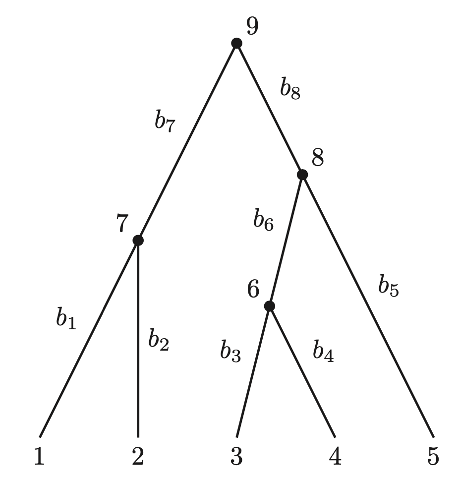
   • If internal node states $ \mathbf{s_Y} $ are known, the likelihood of the site pattern is: \(\begin{align*} \Pr\{\mathbf{s_V} | g\} &= \pi_{s_9} \prod_{(i,j)} p_{s_i,s_j}(b_j) \\ &= \pi_{s_9} p_{s_9, s_7}(b_7) p_{s_7, s_1}(b_1) p_{s_7, s_2}(b_2) \\ &\quad \times p_{s_9, s_8}(b_8) p_{s_8, s_5}(b_5) p_{s_8, s_6}(b_6) p_{s_6, s_3}(b_3) p_{s_6, s_4}(b_4). \end{align*}\)

     where $ \pi_{s_9} $ is the prior probability of the root state, and $ p_{s_i,s_j}(b_j) $ is the transition probability along branch $ b_j $.

2. Likelihood with Unknown Ancestral States:
   • Summing over all possible $ \mathbf{s_Y} $ gives the likelihood of the leaf data: \(\begin{align*} \Pr(\mathbf{s} | g) &= \sum_{S_Y}Pr\{\mathbf{s_V} | g\}\\ &= \sum_{s_9 \in C} \sum_{s_8 \in C} \sum_{s_7 \in C} \sum_{s_6 \in C} \pi_{s_9} p_{s_9, s_7}(b_7) p_{s_7, s_1}(b_1) p_{s_7, s_2}(b_2) \\ &\quad \times p_{s_9, s_8}(b_8) p_{s_8, s_5}(b_5) p_{s_8, s_6}(b_6) p_{s_6, s_3}(b_3) p_{s_6, s_4}(b_4). \end{align*}\)
3. Efficient Reformulation:
   • The summations can be grouped to mirror the tree’s topology, reducing redundant calculations: \(\begin{align*} \Pr(\mathbf{s} | g) &= \sum_{s_9 \in C} \pi_{s_9} \Bigg\{ \sum_{s_7 \in C} p_{s_9, s_7}(b_7) \Big[ p_{s_7, s_1}(b_1) \Big] \Big[ p_{s_7, s_2}(b_2) \Big] \Bigg\} \\ &\quad \times \Bigg\{ \sum_{s_8 \in C} p_{s_9, s_8}(b_8) \Big[ p_{s_8, s_5}(b_5) \Big] \Bigg[ \sum_{s_6 \in C} p_{s_8, s_6}(b_6) \Big( p_{s_6, s_3}(b_3) \Big) \Big( p_{s_6, s_4}(b_4) \Big) \Bigg] \Bigg\}. \end{align*}\)
4. Partial Likelihoods:
   • Define $ L_{i,c} $ as the partial likelihood of data under node $ i $, given its state is $ c $.
   • At each internal node $ y $, the partial likelihood for state $ c $ (denoted $ L_{y,c} $) is computed by combining the likelihoods from the two descendant nodes $ j $ and $ k $.
   • For internal node $ y $ with branches $ (y,j) $ and $ (y,k) $: \(L_{y,c} = \left[ \sum_{x \in C} p_{c,x}(b_j) L_{j,x} \right] \cdot \left[ \sum_{x \in C} p_{c,x}(b_k) L_{k,x} \right].\)
   • Explanation of Terms:
     • $ p_{c,x}(b_j) $: Transition probability from state $ c $ at node $ y $ to state $ x $ at descendant node $ j $, over branch $ b_j $.
     • $ L_{j,x} $: Partial likelihood for descendant node $ j $, assuming state $ x $.
     • The summation $ \sum_{x \in C} $ sums over all possible states ($ A, C, G, T $) for descendant nodes $ j $ and $ k $.
   • For leaf node $ i $: \(L_{i,c} = \begin{cases} 1, & \text{if } c = s_i, \\ 0, & \text{otherwise}. \end{cases}\)
5. Computational Efficiency:
   • Partial likelihoods are computed row by row, avoiding redundant summations.

   • Complexity per site is $ O(n S^2) $, where $ n $ is the number of taxa and $ S =

     C

     $ is the number of character states.

   • The algorithm is linear in the number of taxa and quadratic in the number of states.

The molecular clock

Time-trees and evolutionary rates

• In Chapter 2, we explored several natural tree prior distributions, such as the coalescent and birth–death families, which generate time-trees rather than unrooted trees. But how do these time-trees align with the genetic differences between sequences discussed in Chapter 3? The solution lies in the application of a molecular clock.

The molecular clock

• The molecular clock is a stochastic. Each “tick” of the clock occurs after a stochastic waiting time, determined by the substitution rate $ \mu $.

• Let $ D(t) $ represent a random variable for the number of substitutions that occur over evolutionary time $ t $.

• The probability of exactly $ k $ substitutions occurring in time $ t $ follows a Poisson distribution: \(\Pr\{D(t) = k\} = \frac{e^{-\mu t} (\mu t)^k}{k!}.\)

• In a Poisson process, it is dependent on $\mu t$, the expected number of substitutions per site, $\mu$ and $t$ are unidentifiable without additional information.

Relaxing the molecular clock

• Relaxed molecular clock models allow variation in the rate of molecular evolution among lineages, accommodating non-clock-like relationships.
• Bayesian Framework for Relaxed Molecular Clock:
  • Substitution rates ($ r $) vary across branches using a Bayesian hierarchical approach: \(f(g, \vec{r}, \theta | D) = \frac{\Pr(D | g, \vec{r}, \theta) f(\vec{r} | \theta, g) f(g | \theta) f(\theta)}{\Pr(D)},\) where:
    • $ \vec{r} $: Vector of substitution rates for branches.
    • $ g $: Tree structure.
    • $ \theta $: Other model parameters (e.g., rate distribution parameters).
• Branch-Specific Rate Modeling:
  • The density $ f(\vec{r} | \theta, g) $ can be broken into branch-specific rates: \(f(\vec{r} | \theta, g) = \prod_{\langle i,j\rangle \in R} f(r_{j} | \Phi),\) where $ \Phi $ represents the distribution parameters for rates.
• There is ongoing controversy regarding the assumptions underlying relaxed clock models.”

Autocorrelated Substitution Rates Across Branches

1. Geometric Brownian Motion Model:
   • Introduced by Thorne et al. (1998) to model autocorrelated substitution rates across branches.
   • Defines the probability density of substitution rates ( f(r_i | \mu_R, \sigma^2) ) as: \(f(r_i | \mu_R, \sigma^2) = \frac{1}{r_i \sqrt{2\pi \tau_i \sigma^2}} \exp \left\{ -\frac{1}{2 \tau_i \sigma^2} \left( \ln \left( \frac{r_i}{r_A(i)} \right) \right)^2 \right\},\) where:
     • ( r_i ): Substitution rate for branch ( i ).
     • ( r_A(i) ): Rate of the parent branch.
     • ( \tau_i ): Time separating branch ( i ) from its parent.
     • ( \sigma^2 ): Variance parameter controlling the degree of autocorrelation.
2. Definition of ( \tau_i ):
   • Originally defined as the time between the midpoint of branch ( i ) and the midpoint of its parent branch: \(\tau_i = t_{A(i)} + b_{A(i)}/2 - (t_i + b_i/2),\) where:
     • ( t_i ): Time of the tip-ward node of branch ( i ).
     • ( b_i = t_{A(i)} - t_i ): Length of branch ( i ).
3. Bias-Corrected Model:
   • Kishino et al. (2001) modified the approach by associating a rate ( r_i’ ) with the tip-ward node and defining a bias-corrected geometric Brownian motion model: \(f(r_i' | \mu_R, \sigma^2) = \frac{1}{r_i' \sqrt{2\pi b_i \sigma^2}} \exp \left\{ -\frac{1}{2 b_i \sigma^2} \left( \ln \left( \frac{r_i'}{r_A(i)} \right) + \frac{b_i \sigma^2}{2} \right)^2 \right\}.\)
   • The correction term ( \frac{b_i \sigma^2}{2} ) ensures that the expectation of the child rate matches the parent rate.
4. Average Rate Definition:
   • Instead of directly using ( r_i’ ) as the rate for branch ( i ), Kishino et al. (2001) defined the rate as the arithmetic mean: \(r_i = \frac{r_i' + r_A(i)}{2}.\)
5. Other Models:
   • Variations of autocorrelated clock models include:
     • Compound Poisson Process (Huelsenbeck et al. 2000): Draws rate multipliers ( r_i ) from a Poisson distribution.
     • Thorne-Kishino Model (Thorne and Kishino 2002): Draws ( r_i ) from a log-normal distribution with mean ( r_A(i) ) and variance proportional to branch length.

Uncorrelated Substitution Rates Across Branches

Random Local Molecular Clocks (RLC)

1. Concept:
   • Local molecular clocks divide a phylogenetic tree into regions where substitution rates are consistent within a region but can differ between regions.
   • Unlike strict molecular clocks, these models allow for localized rate changes along branches.
2. Challenges in Early Models:
   • Early applications did not account for:
     • Uncertainty in the phylogenetic tree topology.
     • The number of local clocks.
     • The phylogenetic positions of rate changes.
3. Bayesian RLC Model:
   • Developed by Drummond and Suchard (2010), this model incorporates uncertainty and averages over all possible local clock configurations.
   • For a rooted tree with ( 2n - 2 ) branches:
     • One rate change yields ( 2n - 2 ) possible placements.
     • Two rate changes yield ( (2n - 2) \times (2n - 3) ) placements.
     • Total configurations: ( 2^{2n-2} ), which grows exponentially with ( n ).
4. Parameterization:
   • The RLC model uses:
     • ( \Phi = {\phi_1, \phi_2, \ldots, \phi_{2n-2}} ): Rate modifiers.
     • ( \mathbf{B} = {\beta_1, \beta_2, \ldots, \beta_{2n-2}} ): Binary indicators where ( \beta_i = 1 ) indicates a rate change.
   • Two model flavors:
     • First Flavor: \(r_i = \begin{cases} r_{A(i)}, & \text{if } \beta_i = 0, \\ \phi_i, & \text{otherwise}. \end{cases}\)
     • Second Flavor: \(r_i = \begin{cases} r_{A(i)}, & \text{if } \beta_i = 0, \\ \phi_i \times r_{A(i)}, & \text{otherwise}. \end{cases}\)
5. Autocorrelation and Priors:
   • The second flavor retains autocorrelation in substitution rates between branches.
   • Priors:
     • Elements of ( \Phi ) can follow log-normal distributions (uncorrelated RLC) or gamma distributions (autocorrelated RLC).
   • ( K ), the number of rate changes, is defined as: \(K = \sum_{i=1}^{2n-2} \beta_i,\) with a truncated Poisson prior: ( K \sim \text{Truncated-Poisson}(\lambda) ).
6. Implementation Challenges:
   • Normalizing substitution rates across the phylogeny.
   • Managing differences in model dimensionality during sampling.
   • Requires a Bayesian framework for proper inference.

Branch Rates vs. Site Rates

1. Branch Rates ((r_i)):
   • Represent substitution rates specific to branches in the phylogenetic tree.
   • Constant across all rate categories but vary between branches.
   • Scale the branch length for lineage-specific rate variation.
2. Site Rates ((r_c)):
   • Represent substitution rates specific to different sites in the sequence.
   • Modeled across rate categories (e.g., using a gamma distribution).
   • Capture site-specific rate heterogeneity.
3. Combination:
   • For a given rate category ((r_c)) and branch ((i)), the branch length is scaled by both the branch rate ((r_i)) and site rate ((r_c)): \(\text{Scaled branch length} = r_c \times r_i \times \text{branch length}.\)

Calibrating the molecular clock

Node dating

1. Concept:
   • Node dating uses the geological age of a fossil as a calibration point for phylogenetic divergence in molecular clocks.
   • A calibration density is applied to capture uncertainty in associating fossils with divergence events.
2. Challenges:
   • Reliance on Fossil Evidence:
     • Fossils are used indirectly to determine which molecular divergence they correspond to.
   • Determining Calibration Density:
     • Requires defining the exact form of the calibration density.
   • Assumptions About Node Correspondence:
     • Assumes that fossils correspond directly to a node in the molecular phylogeny, not to an extinct offshoot or ancestor.
3. Improvements:
   • Calibration densities can be enhanced using:
     • Stochastic simulations with phylogenetic speciation and extinction models.
     • Monte Carlo-based methods to construct model-based calibration densities.
4. Bayesian Challenges:
   • Incorporating fossil calibration densities into Bayesian tree priors is computationally challenging when simultaneously inferring the phylogenetic tree.
5. Key Insight:
   • Node dating remains a standard approach but faces significant challenges in accurately integrating fossil evidence into molecular phylogenies.

Leaf Dating

1. Concept:
   • Leaf dating uses differences in sampling dates of sequenced taxa for direct molecular clock calibration.
2. Data Types:
   • Relies on molecular data termed serially sampled, time-stamped, or heterochronous sequences.
   • Such data originates from measurably evolving populations.

Total-Evidence Leaf Dating

• Incorporates fossil taxa as leaves in a phylogenetic time-tree using morphological data.
• Fossil ages are determined based on geological strata, and uncertainties in fossil placement are modeled with MCMC methods.
• Addresses limitations of node dating by directly estimating phylogenetic placement using morphological data.
• Assumes fossils represent ‘extinct offshoots,’ addressing some but not all shortcomings of node dating.

Total-Evidence Dating with Fossilized Birth–Death (FBD) Tree Prior:

• Refines total-evidence dating by introducing the FBD model, which accounts for:
  1. Fossil taxa that are direct ancestors of other taxa (fossil or extant).
  2. Fossil taxa that are extinct offshoots with no direct descendants.
• Utilizes Bayesian MCMC to sample from possible phylogenies, integrating fossil and extant taxa.
• Enables automatic classification of fossils into the two categories, providing a more comprehensive framework for phylogenetic estimation.

Structured trees and phylogeography

Statistical phylogeography

• Phylogeography combines phylogenetics and biogeography to explore geographical and evolutionary relationships.
• Early methods focused on reconciling discrete geographic locations with phylogenetic trees, such as maximum parsimony, but lacked probabilistic uncertainty assessments.
• The transition to model-based approaches paralleled advances in statistical phylogenetics. This shift was supported by the development of Approximate Bayesian Computation (ABC) techniques.
• Statistical phylogeographic methods:
  • Include models that infer geographic states conditional on a phylogenetic tree or jointly estimate phylogeny, geographic states, and parameters.
  • ABC plays a significant role where full Bayesian approaches are impractical, though Bayesian models remain preferred when available due to lower variance.
• The focus is on integrating model-based methods with multi-type branching processes for phylogeographic inference.

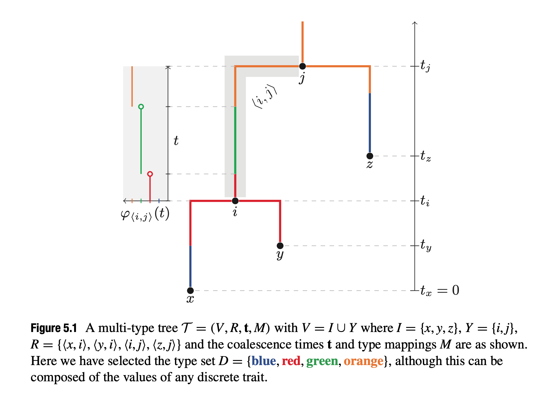
Multi-type trees

• Mathematical Structure:
  • $\mathcal{T} = (V, R, t, M)$:
    • $V$: Set of $2n - 1$ nodes.
    • $R$: Directed edges between nodes $(i, j)$.
    • $t$: Ages of nodes, $t_i \in t$.
    • $M$: Type mappings, $M = {\varphi_{(i,j)} \mid (i, j) \in R}$.
  • Nodes are partitioned into:
    • $I$: External nodes (leaves).
    • $Y$: Internal nodes with:
      • One parent node $i_p$ where $t_{i_p} > t_i$.
      • Two child nodes satisfying $t_{i_c} < t_i$.

• Key Feature: The type function $\varphi_{(i,j)}(t)$ assigns a specific type from $D$ to each edge $(i, j)$ over time $t$. This type mapping allows for the integration of discrete traits (e.g., geographical regions or traits) within the tree structure.

• 

Bayesian Inference of Multi-Type Trees:

1. Inference approaches vary based on:
   • The statistical structure of the multi-type tree model.
   • Specific aspects of the model being inferred.
2. Some models assume independence of multi-type processes on tree edges, enabling efficient integration over type-change events.
   • Example: Migration models assume a fixed time-tree for phylogenetic likelihood calculation.
3. For models not assuming independence, MCMC inference is used for the full multi-type tree, including random type transition events.

Mugration models

1. A mugration model is a mutation or substitution model used to analyse a migration process.
2. Analyze geographic movement of lineages through a continuous-time Markov process.
   • State space represents locations where sequences were sampled.
3. Applications:
   • Estimation of migration rates between location pairs.
   • Reconstruction of ancestral locations on phylogenetic trees.
   • Bayesian stochastic variable selection (BSVS) identifies dominant migration routes.
4. Contributions:
   • Helped investigate origins and global spread of Influenza A H5N1 and H1N1.
   • Improved estimation by addressing spatial and temporal sampling density.
5. Challenges:
   • Limited to pre-defined sampling locations.

The stuctured coalescent

• 
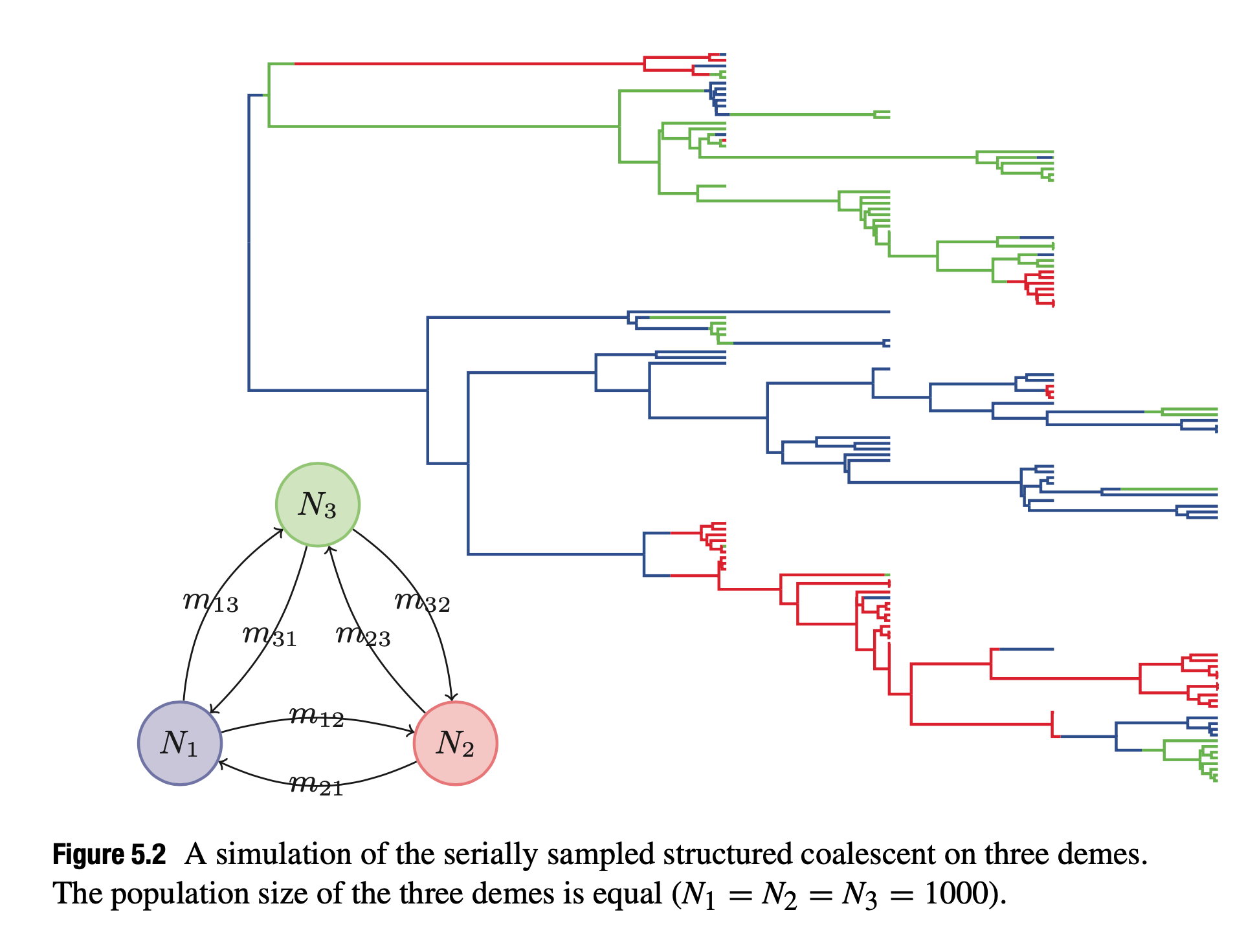
• Concept: The structured coalescent (Hudson 1990) is applied in phylogeography to estimate migration rates between subpopulations or “demes” over time.
• Applications:
  • Initially used for analyzing subpopulations (e.g., HIV dynamics) or host populations (Ewing et al. 2004).
  • Allows Bayesian and maximum likelihood frameworks for subpopulation sizes and migration rates estimation.
  • Extensions include heterochronous samples and ghost deme effects.
• Challenges:
  • Computational demands due to integrating genealogical tree and migration parameters (one ad hoc solution is the mugration mode, which assumes the migration process is independent of the coalescent prior).
  • Efforts such as “uniformisation” aim to simplify Bayesian MCMC sampling.

Structured Birth-Death Models

• Concept: Extends the birth-death process (Kendall 1949) to account for structured population dynamics, incorporating migration among discrete demes.
• Features:
  • Migration events occur along branches of phylogenies when samples represent different geographic locations.
  • Type changes at branching events capture events like superspreaders in epidemics.
• Inference Approaches:
  • Multi-type trees can integrate migration events.
  • Alternatively, migration events can be integrated out for standard BEAST trees.
• Applications in Epidemics:
  • Reconstruct epidemiological parameters, such as the effective reproduction number $ R $, differing among demes.

Phylogeography in a spatial continuum

• Spatial aspects of samples can be modeled as a continuum using diffusion models, which are suited for viral spread and host movement.
• Example: Rabies virus geographic expansion in the U.S. and the phylogeography of feline immunodeficiency virus in cougars (Puma concolor).
• Brownian diffusion models have been widely used but assume rate homogeneity across branches, which can be limiting.
• Relaxed diffusion models (Drummond et al., 2006; Lemey et al., 2010) extend the relaxed clock concept, showing improved coverage and efficiency over Brownian diffusion.
• These models focus on spatial movement resembling an over-dispersed random walk but ignore population density and geographic spread interactions in genealogies (like mugration).

Phylodynamics with structured trees

• Phylodynamics integrates mathematical epidemiology and statistical phylogenetics to model the evolution and population dynamics of pathogens.
• Particularly effective for viral and bacterial pathogens due to rapid evolution observable within short timeframes (weeks to years).
• Early efforts in phylodynamics include:
  1. Deterministic Models: Modelling pathogen population sizes through time (Volz et al. 2009, 2012).
  2. Transmission Tree Models: Developing new models suited to pathogen spread and sampling dynamics (Stadler et al. 2013).
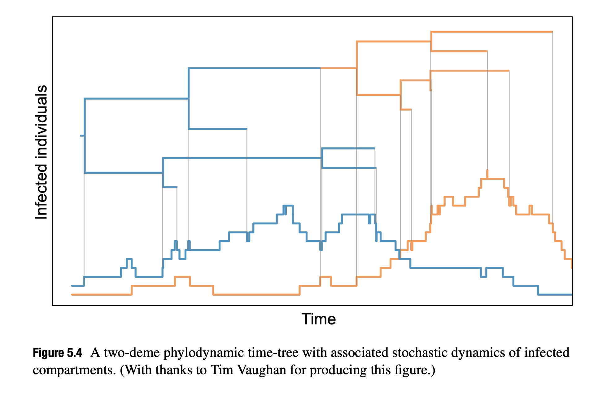
  3. Stochastic Models: Coupling transmission models with stochastic compartmental models for epidemics (Kühnert et al. 2014).
• The structured SIR process (Figure 5.4) depicts two demes undergoing stochastic SIR processes. Events in the phylogenetic tree correspond to changes in infected population trajectories.
• 

Conclusion

• Structured models in phylogenetics associate each branch with a specific type, forming jump processes as types transition along branches.
• Simple models assume independence in jump rates across branches, while complex models couple jump processes with co-evolving stochastic processes.
• Bayesian inference methods remain under development for these models, but their application is growing due to the active research in this area.