I wanted to get in more details about the structured coalescent model, here I record some notes when I read related papers/tutorials, and watch videos.

Coalescent quick recap

It is a series of short Youtube videos by Scott Roy.

• Coalescent is about mathematically trace back in time to find a appropriate tree shape / genealogy that can explain the observed data.
• Geometric Series Summation: $\sum_{i=0}^{\infty}{r^i} = \frac{1}{1-r}$ (note that $0<r<1$, and r can be a probability of coalescence). So that $\sum_{i=0}^{\infty}{(1-p)^i} = \frac{1}{p}$.
• Time for $n=2$ individuals to coalescence is a classic waiting problem: \(P(t)=(\frac{N-1}{N})^{t-1}\frac{1}{N}\\ E(t)=\frac{1}{\frac{1}{N}}=N\)

• Expected waiting time for coalescence (discrete):

  \[\begin{align*} E[t] &= 1p+2p(1-p)+3p(1-p)^2+... \\ &=\sum_{i=0}^{\infty}{(i+1)p(1-p)^i} =\sum_{i=1}^{\infty}{ip(1-p)^i} =\sum_{i=0}^{\infty}{ip(1-p)^i}\\ &=\sum_{i=0}^{\infty}{ip(1-p)^i} + \sum_{i=0}^{\infty}{1p(1-p)^i}\\ &=(1-p)\sum_{i=0}^{\infty}{ip(1-p)^{i-1}}+p\sum_{i=0}^{\infty}{(1-p)^i}\\ &=(1-p)E[t]+p\frac{1}{p}\\ &=\frac{1}{p} \end{align*}\]
• Time for $n>2$ individuals to coalescence:
  • First coalescence:
  \[E(t)=\frac{1}{\frac{n\choose2}{N}}=\frac{N}{n\choose2}\]
  • Second coalescence:
  \[E(t)=\frac{N}{n-1\choose2}\]
  • Third coalescence:
  \[E(t)=\frac{N}{n-2\choose2}\]
  • …
  • Such that the coalescence time is getting longer for deep branches.

• To jointly model mutation process and coalescent process, we need to consider the mutation rate $\mu$ and coalescent rate $\lambda$. The expected number of mutations before the first coalescence is:

  \[\begin{align*} E(mut)&=\frac{\mu}{\lambda}\\ &=\frac{n\mu}{n\frac{n\choose2}{N}}\\ &=\frac{2N\mu}{n-1}. \end{align*}\]

  As a result, the expected number of mutations increases backwards in time (as $n$ is decreasing).

• Coalescent frequency site distribution can be obtained as a neutral model for genetic variation. Comparing the observed FSD with the expected FSD can help to infer the selection pressure.
• The expected number of singletons and the expected ratio between the number of singletons and the number of SNPs surprisingly can be represented by simple formulas, after canceling out the terms. These can be useful for inferring evolutionary history.
• The probability of particular coalescent tree shapes can also be calculated, often also resulted in simple formulas, as exampled here.
• There is also ways to work out the probability and expected tree lengths for coalescent subdivisions, as exampled here. After getting the formula numerically, we can easily tell what will happen e.g. if migration rates is much higher than the coalescent rate (or vice versa).

Coalescent theory by John Wakeley on a workshop (Second Bangalore School on Population Genetics and Evolution)

This is a quite old series of lectures, but should be relevant.

Basic Probability theory

• Using an example from a Nature paper on 2001: A map of human genome sequence variation containing 1.42 million single nucleotide polymorphisms, where they sampled 12027 loci, with each loci spanning ~500bp. They get a summarized table of the number of SNPs in different frequency classes. The data can be used to infer the demographic history of human populations. One need to use a random model to explain the observed data.

  #SNPs	#loci	Proportion of loci
  0	8796	0.731
  1	2247	0.187
  2	668	0.056
  3	214	0.018
  4	102	0.008

• In this lesson, he recalled concepts of probability theory, including expectation, variance, Bernoulli/Binomial random variables. In a Wright-Fisher model, the number of copies of a particular allele in a population is a binomial random variable. The expected number of copies of a particular allele in a population is $2Np$, and the variance is $2Np(1-p)$.
• $Binomial(n,p) \approx Poisson(np)$ when $n$ is large and $p$ is small, and $np$ becomes \(\lambda\). $P(K=k)=\frac{\lambda^k}{k!}e^{-\lambda}$, $E(K)=\lambda$, $Var(K)=\lambda$.
• Geometric random variable (waiting time of Binomial trials) has $P(K=k)=(1-p)^{k-1}p$, $E(K)=\frac{1}{p}$, $Var(K)=\frac{1-p}{p^2}$.
• Exponential random variable (waiting time of Poisson events) has $P(K=k)=\lambda e^{-\lambda k}$, $E(K)=\frac{1}{\lambda}$, $Var(K)=\frac{1}{\lambda^2}$.

Gene genealogies and coalescent processes

• A starting example in this lesson is a Nature paper from Li Heng in 2011: Inference of human population history from individual whole-genome sequences. They estimate the effective population size of human populations using the coalescent theory. They also modeled recombination in the coalescent process.
• Some measures of variations:
  • $S$: number of segregating sites.
  • $\pi$: Nucleotide diversity: average pairwise difference.
  • $Z_i$: (Unfolded) Site frequency spectrum, number of sites with $i$ copies of mutant.
  • $\eta_i$: Folded Site frequency spectrum: number of polymorphic sites where the less-frequent (minor allele) allele has frequency $i$.
• The coalescent, notations:
  • Sample size: $n$.
  • Population size: $N$.
• Number of generations to a coalescent event: $P(G=g)=(1- \frac{n\choose2}{2})^{g-1}\frac{n\choose2}{2}$ as a geometric random variable. Or $f_{T_{n}}(t)={n\choose2}e^{-{n\choose2}t}$ as an exponential random variable, where one unit of time is $N$ generations.
• Expected Number of Segregating Sites:
  • $E[S]=\sum_{i=2}^{n}i\cdot E[T_i]\cdot \theta$:
    • $i$: Number of lineages in a coalescent interval.
    • $E[T_i]$: Expected coalescent time for $i$ lineages, $\frac{2}{i(i-1)}$, note that this is in units of $N$ generations.
    • $\theta$: Scaled mutation rate.
  • Simplified formula: $E[S]=\theta \sum_{i=2}^{n}\frac{1}{i-1}=\theta \sum_{i=1}^{n}\frac{1}{i}$.
• Expected total number of mutations:
  • $K$ follows a Poisson distribution with mean $\frac{\theta}{2}$, where $\theta = 4N_e\mu$ is the scaled mutation rate.
  • $P(K = k \mid \theta) = \frac{\left(\frac{\theta}{2}\right)^k e^{-\frac{\theta}{2}}}{k!}$
    • Describes the probability of observing $k$ mutations.
• Number of Mutations Between Two Sequences ($K_2$)
  • Coalescent Time Distribution:
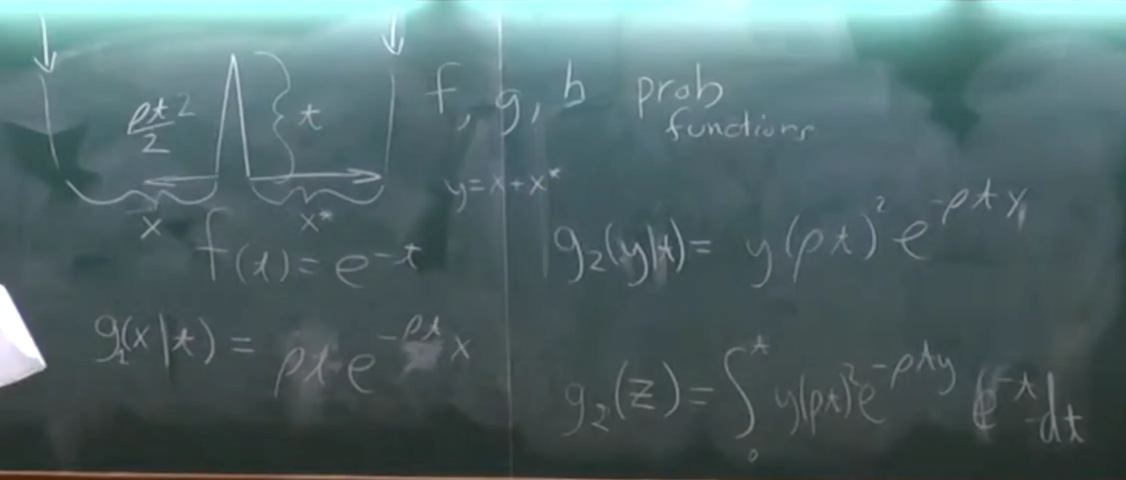
    • The coalescent time $T_2$ follows an exponential distribution with mean $1$ (in coalescent units): $f_{T_2}(t) = e^{-t}.$
  • Conditional Probability of Mutations Given $T_2$:

    • $K_2$ (number of mutations) follows a Poisson distribution conditioned on $T_2$, with mean $\frac{\theta t}{2}\times 2$:

      \[P(K_2 = k \mid T_2 = t) = \frac{\left(\theta t\right)^k e^{-\theta t}}{k!}.\]

    • Describes the probability of observing $k$ mutations, given coalescent time $T_2 = t$.

  • Unconditional Probability of Mutations:

    • Marginalizing over all possible $T_2$ values, the probability of $K_2 = k$ is:

      \[P(K_2 = k) = \int_0^\infty f_{T_2}(t) \cdot P(K_2 = k \mid T_2 = t) \, dt.\]

    • Combines the exponential distribution of $T_2$ with the Poisson mutation process.

  • Resulting Probability:

    \[P(K_2 = k) = \left(\frac{\theta}{\theta + 1}\right)^{k} \cdot \frac{1}{\theta + 1}\]
  • $\theta$: Scaled mutation rate ($4N_e\mu$).
  • Can be viewed as a geometric distribution with parameter $\frac{1}{\theta + 1}$ (waiting problem for multiple mutations and a final coalescent).

Gene genealogies with recombination

• Recall the the expected number of segregating sites: $E[S]=\theta \sum_{i=1}^{n}\frac{1}{i}$.
• Note that the expected nucleotide diversity $\pi$ is the average pairwise difference, which is $E[\pi]=\theta$, which is the same as the expected number of segregating sites when $n=2$.
• Expected site frequency spectrum: $E[Z_i]=\frac{\theta}{i}$.
• Tajima’s D compares two estimates of genetic diversity to infer deviations caused by selection, demographic events, or other evolutionary processes.
• Recombination complicates coalescent theory because it causes different parts of the genome to have different genealogies, breaking the simple tree-like structure of the standard coalescent process.
  • 

• Covariance Between Coalescent Times ($T_1, T_2$):

  \[\text{Cov}[T_1, T_2] = \frac{\rho + 18}{\rho^2 + 13\rho + 18}\]
  • $T_1, T_2$: Coalescent times for two loci.
  • $\rho = 4N_e r$: Scaled recombination rate.
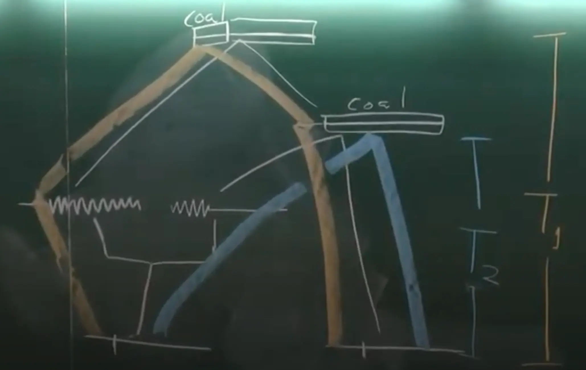
• Sequential Markov Coalescent (SMC), is a computationally efficient approximation to the full Ancestral Recombination Graph (ARG). The SMC framework models the genealogy of sequences along a genome, incorporating recombination to simulate how local genealogies change sequentially along the genome.
  • Instead of modeling the entire recombination history, the SMC assumes a Markovian process for genealogies along the genome.
  • Along the genome, recombination causes the genealogical tree to “switch” to a new topology at certain points.
  • These switches happen at recombination breakpoints and are shown in the diagram as transitions between trees.
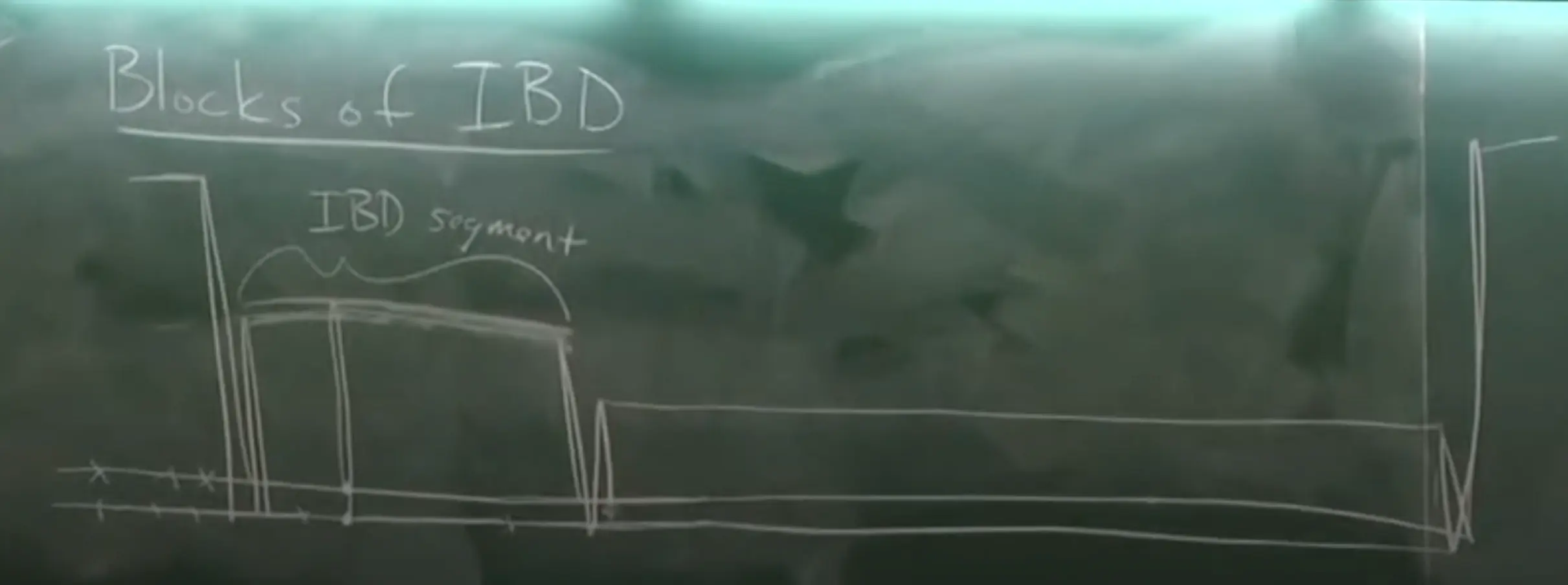
• Identity by Descent (IBD) occurs when two or more genetic segments in different individuals are inherited from a common ancestor without any intervening recombination or mutation. These segments are identical because they have been directly passed down through generations from the same ancestor.
• IBD can also be view distributed along a genome:
  • 
• We can also model within the IBD segment, giving a focal point:
  • 

Structured coalescent

• Non-exchangeability of lineages in structured populations:
  • In structured populations, lineages are not exchangeable because they are more likely to coalesce with lineages from the same subpopulation.
  • This non-exchangeability affects the coalescent process and the genealogies of sequences.
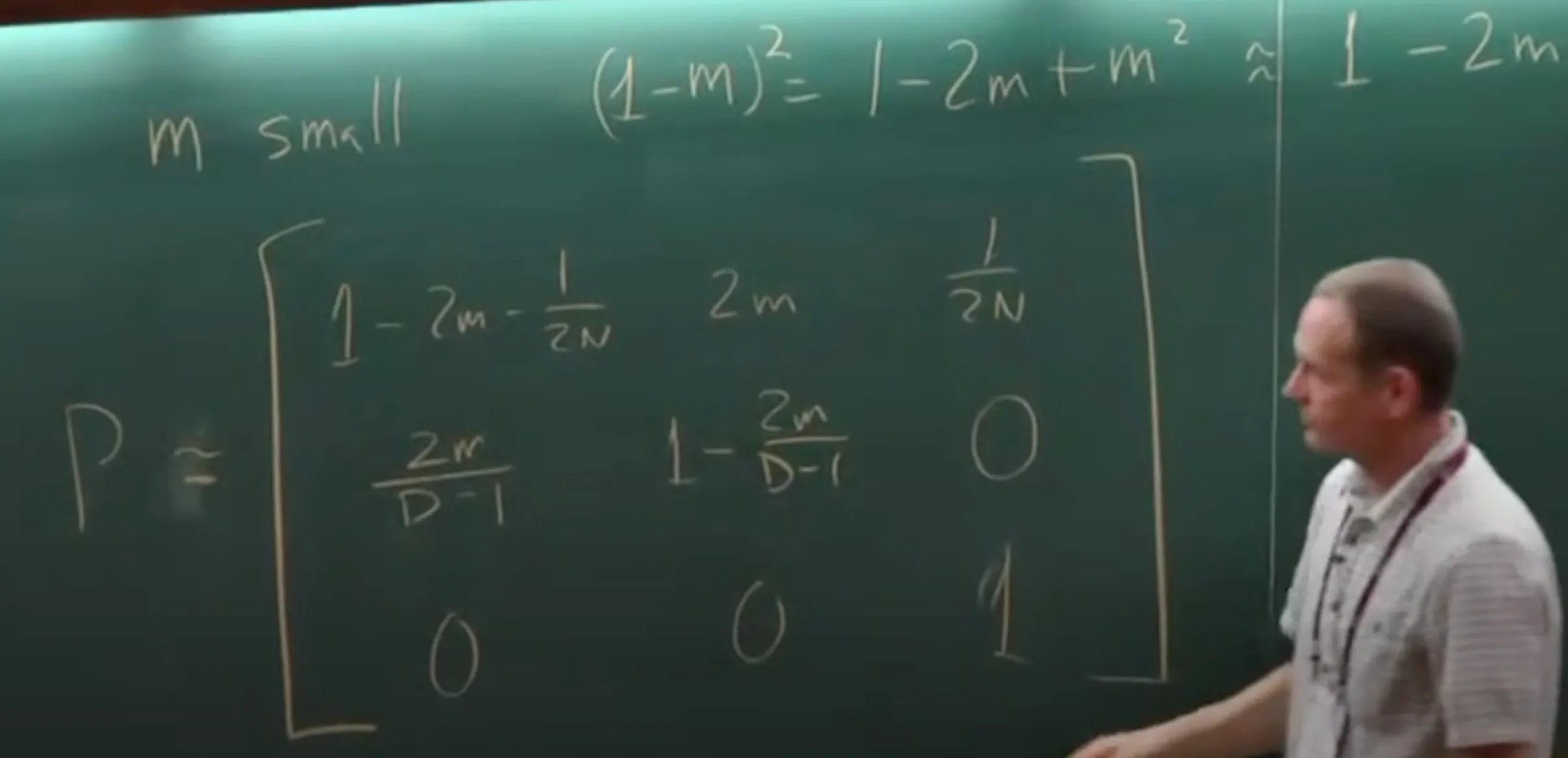
• He revisit the Markov chain model, specified with a transition probability matrix.
  • This matrix describes the probability of transitioning between states (generations) in the Markov chain, with each $P$ representing the probability of transitioning from one state (generation with $i$ lineages) to another state (generation $i-1$ lineages).
• Recall that, based on Wright–Fisher (discrete‐generation) model, $P(i \to i-1) = \frac{\binom{i}{2}}{2N} \prod_{k=2}^{i-1} \left(1 - \frac{k}{2N}\right)$ is the probability that, in the next generation, exactly one pair of the $i$ current lineages coalesces (merges), resulting in $i−1$ distinct ancestral lineages (all the others do not coalesce).
  • If we multiply this by $2N \to\infty$, we get $i\choose2$, this result in the coalescent rate in the time scale of $2N$ generations.
• Wright’s Island Model:
  • Notations:
    • $D$: demes (subpopulations).
    • $N$: deme size
    • $m$: migration probability (equally likely to every other deme).
  • When $n=2$, the instantaneous transition matrix (for how long does it take to coalesce) can be derived:
    • State 1: both lineages are in the same deme.
    • State 2: lineages are in different demes.
    • State 3: lineage coalesced.
    • 
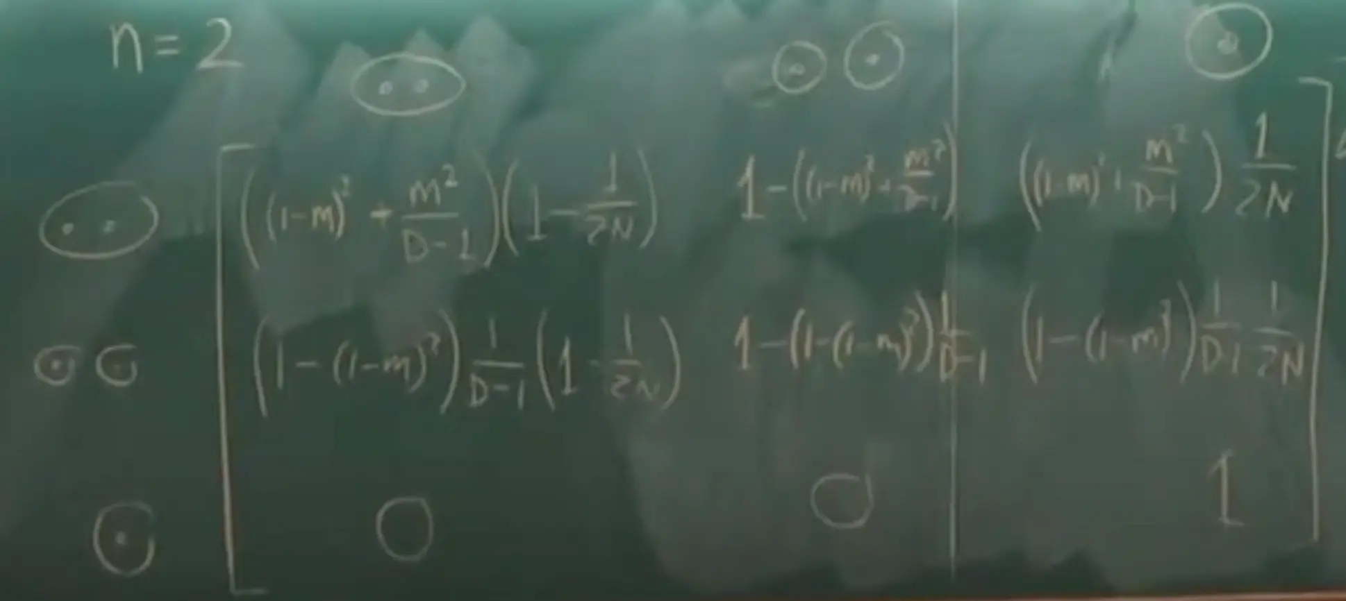
  • If $m\to0$ in this matrix, we can ignore the $m^2$ terms, then we have:
    • 

  • It can be further simplified to the below matrix, if multiplied by $2N$:

    \[Q = \begin{bmatrix} -M - 1 & M & 1 \\ \frac{M}{D - 1} & -\frac{M}{D - 1} & 0 \\ 0 & 0 & 1 \end{bmatrix}\]
  • The waiting time in state 1 is $f_1(t)=(M+1)e^{-(M+1)t}$, with $E[T_1]=\frac{1}{M+1}$.
  • The waiting time in state 2 is $f_1(t)=(\frac{M}{D - 1})e^{-(\frac{M}{D - 1})t}$, with $E[T_2]=\frac{D-1}{M}$.

  • $T_w$: Coalescent time (within) started from state 1:

    \[\begin{align*} E[T_w]&=\frac{1}{M+1}+\frac{M}{M+1}\cdot E[T_b]+ \frac{1}{M+1}\cdot 0 \\ &=D \end{align*}\]

  • $T_b$: Coalescent time (between) started from state 2:

    \[\begin{align*} E[T_b]&=\frac{D-1}{M}+ E[T_w] \\ &=D(1+\frac{D-1}{MD}) \end{align*}\]
  • $T_w$ and $T_b$ can be solved if put together.
• A more relaxed model:
  • Notations:
    • $N_i$: size for deme $i$.
    • $q_{ij}$: migration rate from deme $i$ to deme $j$.
  • The $N_i$ can changed, something similar to the traveler matrix in the metapopulation model is happening.
  • Conservative migration: forwards and backwards migration rates are equal.

Coalescent theory by Aneil Agrawal on a workshop (Fourth Bangalore School on Population Genetics and Evolution)

Drift, Inbreeding, and $N_e$

• Under only genetic drift, The cumulative probability that a coalescence event has occurred by generation $t$: $F(t) = 1/(2N) + (1 - 1/(2N)) * F(t-1) = 1 - (1 - 1/(2N))^t$.
• Considering also the mutation process with $\mu$ rate, $F(t) = 1 - (1 - 1/(2N))^t \cdot (1-\mu)^2$. Assuming equilibrium and assuming $N$ is large, $\mu$ is small, we get $F^*=\frac{1}{4N\mu}=\frac{1}{\theta}.$
• Effective population size is the size of an idealized population that would show the same amount of genetic drift or inbreeding as the population under consideration. Many process cannot be modeled/captured by a single $N_e$.

Coalescence I: basic theory and connection to mol pop gen statistics

• The probability of NOT coalescing (for constant N) in $t$ is $1-F(t) = (1 - 1/(2N))^t$, using first order Taylor expansion ($e^x \approx 1 + x \quad \text{if }

  x

  \ll 1$), we get $1-F(t) \approx e^{-t/(2N)}$.

• The probability of NOT coalescing (for changing N), the probability of NOT coalescing is equivalent to the harmonic mean of the population size over time. Note that harmonic mean is the reciprocal of the average of the reciprocals, which is sensitive to small values.
• Gender bias can lead to less effective population size than the actual population size.
• A model without self-fertilization, which can also yield smaller effective population size than actual population size.
• Smaller effective population size $\approx$ more genetic drift $\approx$ more homozygosity.
• In later part of the lesson, he revisited the (total) time to coalescence for $k$ lineages.
• The expected number of mutations is $2\mu \bar{t}=4N\mu. $

Coalescence II: structured coalescent including pop structure, selfing, and background/balancing selection

• The probability of a mutation events among all events: $\frac{P(mut)}{P(something)}=\frac{2\mu}{2\mu+\frac{1}{2N}}=\frac{4N\mu}{4N\mu+1}=\frac{\Theta_{\pi}}{\Theta_{\pi}+1}$
• Expected number of segregating sites: $E[S]=\Theta_w \sum_{i=1}^{k-1}\frac{1}{i}$.
• Tajima’s D comparing $\Theta_{\pi}$ and $\Theta_w$, by $D=\frac{\Theta_{\pi}-\Theta_w}{\sqrt{Var(\Theta_{\pi}-\Theta_w)}}$. The expectation is zero, if under an idealized Wright-Fisher model. Excessive rare variants (negative $D$) can be due to population expansion, or balancing selection. Excessive common variants (positive $D$) can be due to population contraction, or directional selection.
• Mcdonald-Kreitman test use polymorphism and divergence to infer selection. Considering two species, it takes $G$ generations to reach back to the ancestral specie, and $2N_A$ generation to coalesce (within the ancestral specie), so $T_D=2N_A+G$. The expected number of sequence divergence is $E[D]=2\mu T_D$. In this test, y ou can take the ratio of the number of segregating sites to the number of divergence sites. The ratio should be the same for synonymous and non-synonymous sites, if there is no selection. $\frac{E(S_{syn})}{E(D_{syn})}= \frac{E(S_{non})}{E(D_{non}) }$.
• Kimura’s neutral theory argued that most evolutionary changes in DNA (or amino acid) sequences are the result of random fixation of neutral mutations rather than being driven by natural selection. In other words, while beneficial and deleterious mutations certainly occur, the bulk of the substitutions (i.e., the differences that become fixed between species) are those that are effectively neutral with respect to fitness.
• Strongly deleterious mutations are not likely to be observed in the data, thus not contributing to the number of segregating sites, however, they can contribute to the divergence.

• If we set $a$ as the number of adaptive substitutions, assuming weakly deleterious mutations, thus not affecting $E(S_{non})$ but only affecting $E(D_{non})$, we can get:

  \[\begin{aligned} D_{non} &= 2\mu T_D + a, \\ \\ a &= D_{non} - 2\mu T_D\\ &= D_{non} - E(S_{non})\frac{E(D_{syn})}{E(S_{syn})}. \end{aligned}\]
• The estimation of $a$ is surprisingly high ($\approx 0.4$) for some cases, but for human data it is low.
• In structured populations, the alleles are not exchangeable - quite complicated!

• Rederived the classic coalescent time for two alleles. He constructed the same instantaneous transition matrix as John Wakeley did in the earlier notes.

  \[\begin{aligned} \mathbb{E}[T_1] &= 2\,d\,n,\\ \mathbb{E}[T_2] &= 2\,d\,n \;+\; \frac{d - 1}{2\,m},\\ \mathbb{E}[T_*] &= \frac{1}{d}\,\mathbb{E}[T_1] \;+\; \bigl(1 - d\bigr)\,\mathbb{E}[T_2]. \end{aligned}\]

• FST is a measure of population differentiation due to genetic structure, from a coalescent perspective:

  $$ \begin{aligned} F_{ST}&=\frac{E(H_T)-E(H_S)}{E(H_T)}
  &=\frac{E(T_{})-E(T_1)}{E(T_{})}
  &= \frac{(d - 1)^2}{1 - 2d + d^2 \left(1 + 4mn\right)}\
  \lim_{d\to \infty} F_{ST} &= \frac{1}{1 + 4mn}

  \end{aligned} $$ Note that $mn$ is like the number of migrants per generation. Be careful that there are many assumptions in this model, which are usually not met in real data.